Sinusoidal Steady State Analysis – Electric circuits

In steady state (the fully charged state of the cap), current through the capacitor becomes zero. The sinusoidal steady-state analysis is a key technique in electrical engineering, specifically used to investigate how electric circuits respond to sinusoidal AC (alternating current) signals. This method simplifies the intricate details involved in time-varying AC circuits by representing voltages and currents as phasors—complex quantities that succinctly convey both amplitude and phase information.

What is Sinusoidal Steady State Analysis?

Steady-state means no transients, i.e., after 5-time constants of switching action. Stable-state analysis of A.C. circuits is more conveniently done with the help of phasor representation.

like [Tex]V(t) = V_m \sin(\omega t + \phi) [/Tex]

where Vm denotes amplitude, ω is angular frequency, it signifies time, and ϕ represents the phase angle. To streamline analysis, architects employ phasors—complex figures incorporating breadth and phase information. The phasor fellow of a sinusoidal signal, Vm ∠ ϕ, facilitates algebraic operations and simplifies circuit analysis.

Impedance, akin to resistance in DC circuits, is introduced as the amalgamation of resistance and reactance. The impedance of capacitors (Z_C=1/ωC) and inductors (Z_L=jωL) assumes a pivotal role in assessing AC circuits. This analytical approach proves invaluable in comprehending how circuits react to AC signals at specific frequencies, aiding in the efficient design and optimization of electrical systems

Sinusoidal Source

A sinusoidal source in electrical engineering generates an alternating current (AC) with a sinusoidal waveform. This equation representing a sinusoidal voltage is given by:

[Tex]v(t)= Vm. \sin(\omega t + \phi) [/Tex]

• where v(t) is the instantaneous voltage at time t.
• Vm is the amplitude or peak voltage
• w is the angular frequency
• It is time.
• [Tex]\phi [/Tex] is the phase angle

Derivation of Sinusoidal Steady State Analysis

Since , f=1/T

[Tex]\omega = 2\pi f = \frac{2\pi}{T} [/Tex]

[Tex]v(t)= Vm. \sin(\omega t + \phi) [/Tex]

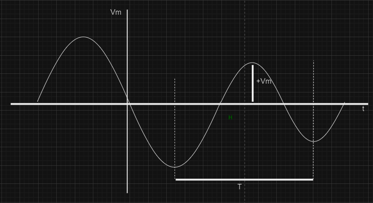
The coefficient of Vm, Vm​ in the above equation represents the maximum amplitude of the sinusoidal voltage, as cosine is confined within the bounds of (+Vm​,−Vm​), encapsulating the amplitude range. The illustrated figure elucidates these characteristics. Meanwhile, the angle Φ is denoted as the phase angle of the sinusoidal voltage. The value is found as the square root of the mean value of the square function

–[Tex]\sqrt{\int_{t_0}^{t_0+T} V_{m} ^2\cos^2(\omega t + \phi) \, dt} [/Tex]

The above equation reduces

[Tex]\frac{V_m^2}{{2}} [/Tex]

Now,

[Tex]V_{\text{rms}} = \frac{V_m}{\sqrt{2}} [/Tex]

Phasor of Sinusoidal Steady State Analysis

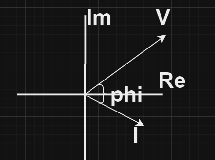
A rotating vector that represents a Sinusoidal -varying quality is called a phasor. Vector will rotate with an angular velocity equal to the angular frequency of that quantity. Its length represents the amplitude of the quantity, and its projection upon a fixed axis gives the instantaneous value of that quantity.

[Tex]V=Vm<\phi [/Tex]

• where V is the phasor representing the voltage
• Vm is the amplitude of the sinusoidal waveform
• [Tex]<\phi [/Tex] is the phase angle.

Derivation of the Phasor

We know that the phasor representation in sinusoidal steady state analysis is for a linear time-invariant system.

So, Assuming the input is a sinusoidal signal,

[Tex]V(t) = V_0 \sin(\omega t + \phi) [/Tex]

[Tex]cosine formate- V(t) = V_0 \cos(\omega t + \phi_o-\pi/2) [/Tex]

using euler’s identities,

[Tex]e^{j\theta} = \cos(\theta) + j\sin(\theta) [/Tex]

[Tex]V_oe^{j(wt + \phi_o – \frac{\pi}{2})} = V_o\cos(wt + \phi_o – \frac{\pi}{2}) + jV_o\sin(wt + \phi_o – \frac{\pi}{2}) [/Tex]

[Tex]V_oe^{j( \phi_o – \frac{\pi}{2})}e^{j(wt)} = V_o\cos(wt + \phi_o – \frac{\pi}{2}) + jV_o\sin(wt + \phi_o – \frac{\pi}{2}) [/Tex]

[Tex]\text{Re}\{V_o e^{j(\phi_o – \frac{\pi}{2})}e^{j\omega t}\} = V_o \cos(wt + \phi_o – \frac{\pi}{2}) =V(t) [/Tex]

where [Tex]V_s=V_o e^{j(\phi_o – \frac{\pi}{2})} [/Tex] = phasor.

Now angle Notation:-

[Tex]1 \angle \phi^\circ = 1e^{j\phi}[/Tex]

Key Terminologies

Time Period: The time period, which means that one complete oscillation will occur, is called the time period.The unit of time period is the second, denoted by T

[Tex]\Tau=2\pi/\omega [/Tex]

Frequency, represented as( f), is an abecedarian aspect of rolling analysis, indicating the number of cycles a periodic waveform completes in one second. Measured in Hz, it’s the antipode of the time period (T).

f =1/T

Angular frequency

[Tex]\omega = 2 \pi f [/Tex]

Sinusoidal Waveform: Sinusoidal is a sine wave, which means that the amplitude of a variable changes with time.who smoothly repeats the oscillation, suggesting the shape of a sine rolling.

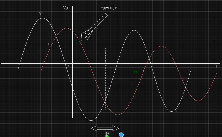
V-I Relation for an Inductor

The voltage-current relationship for an inductor in an electric circuit is described by the following equation:

[Tex]v(t)=L di(t)/dt [/Tex]

• where v(t) is the instantaneous voltage across the inductor at time t.
• L is the inductance of the inductor
• i(t) is the instantaneous current flowing through the inductor.

This equation signifies that the voltage across an inductor is proportional to the rate of change of current with respect to time.

[Tex]V = j\omega LI [/Tex]

then voltage leads the current by 90.

[Tex]V = \omega L I_m \angle (\theta_i + 90^\circ)[/Tex]

Graph of V-I Relation for an Inductor

V-I Relationship for a Capacitor

The voltage-current relationship for a capacitor in an electrical circuit is given by the following equation:

[Tex]i(t)=Cdv(t)/dt [/Tex]

Then,

[Tex]V = \frac{1}{j\omega C} \cdot I [/Tex]

• i(t) is the instantaneous current through the capacitor at time t.
• C is the capacitance of the capacitor.
• v (t) is the instantaneous voltage across the capacitor.
• This equation describes that the current through a capacitor is proportional to the rate of change of voltage with respect to time.
• The voltage across the terminals of a capacitor lags by current.

[Tex]V = \frac{I_m}{\omega C} \angle (\theta_i - 90^\circ)[/Tex]

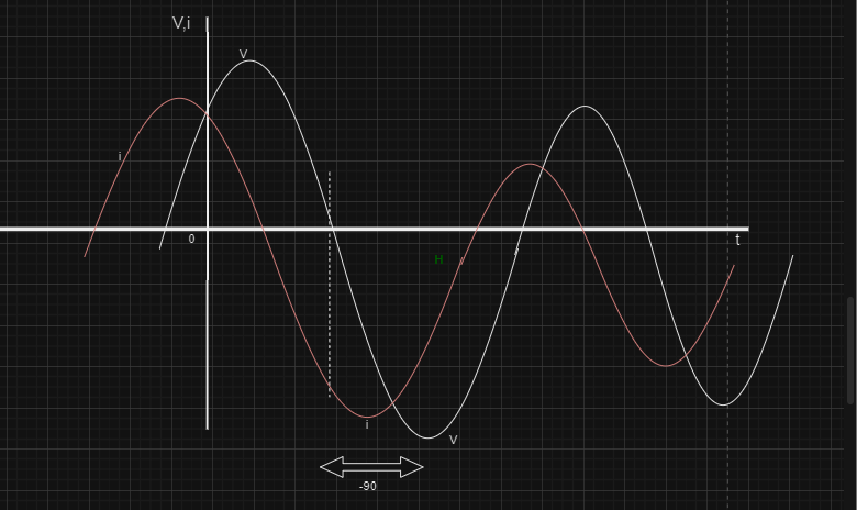
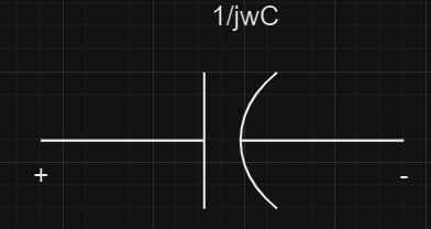
Graph of V-I Relationship for a Capacitor

The graph of the V-I relationship for a capacitor is a phasor-shifted sine wave. When an AC voltage is applied, the current leads the voltage due to capacitors characteristics in the form of an electric field.

Impedance

Impedance is a concept in electric engineering that calculates the opposition a circuit element presents to the flow of alternating current (AC). It is represented by the symbol Z and is a complex quantity with magnitude and phase components.

Z= R + j x X

• where Z is the impedence
• R is the resistance
• X is the reactance
• j is the imaginary unit.

Resistor impedence:

Z=V/i=R

Capacitor impedence:

[Tex]Z= V/i = 1/j\omega C [/Tex]

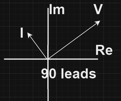
Phaser Diagram: In this the current leads voltage by 90 degree as shown in the diagram also:

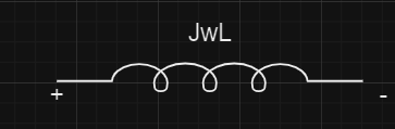
Inductor impedance

Z= V/i=jwL

Phase diagram: current lags voltage by 90

Reactance

Reactance is the imaginary part of impedence and signifies the opposition to the flow of alternating current due to capacitance or inductance in a circuit. Reactance (X) can be classified into capacitive reactance (Xc) and inductive reactance (X_L)L.

Capacitance Reactance

Capacitance reactance is denoted by X_C.

Here, w is the angular frequency, and C is the capacitance.

The negative sign in the capacitive reactance formula indicates that in a capacitor, the current leads the voltage in terms of phase.

Inductance Reactance

Inductance Reactance is denoted by X_L.

The positive sign in the inductive reactance formula signifies that in an inductor, the current lags behind the voltage in terms of phase.

AC (Alternating Current) Power Analysis

Electric power destroyed by a resistance in an AC circuit is different from the power destroyed by a reactance, as reactances do not dissipate energy.

In a DC circuit, the power consumed is simply the product of the DC voltage times the DC current, given in watts. Still, for AC circuits with reactive factors, we’ve got to calculate the consumed power elsewhere.

Also, the power absorbed or supplied by a circuit element is the product of the voltage, V, across the element and the current, I, flowing through it. So if we had a DC circuit with a resistance of “R” ohms, the power dissipated by the resistor in watts would be given by any of the following generalized formulas:

[Tex]P = V \cdot I= \frac{V^2}{R}= I^2 \cdot R [/Tex]

Electric Power in AC Circuit

In a DC circuit, the voltages and currents are generally constant; they aren’t varying with time as there’s no sinusoidal waveform associated with the force. Still, for power in AC circuits, the immediate values of the voltage, current, and thus power are constantly changing due to the force. So we can’t calculate the power in AC circuits in the same manner as we can in DC circuits, but we can still say that power( p) is equal to the voltage( v) times the amperes( i).

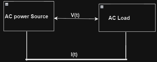
So, in this diagram, the term:

The AC power source defines the source of alternating current while providing a voltage V(t).

AC load defines the electrical load through which current I(t) flows.

This diagram is a fundamental representation and doesn’t include details such as power factor, phase angle, or the relationship between real power and reactive power.

P(t) =V(t) x I (t) that is instantaneous namaste power.

Where

[Tex]V = V_m \sin(wt + \theta_v) [/Tex]

[Tex]i = I_m \sin(wt + \theta_i) [/Tex]

Then

[Tex]P = V_m I_m \sin(wt + \theta_v) \sin(wt + \theta_i) [/Tex]

Apply this,

[Tex]\sin(A) \sin(B) = \frac{1}{2} \left[ \cos(A – B) – \cos(A + B) \right] [/Tex]

[Tex]P = \frac{V_m I_m}{2} \left[ \sin(\theta) – \cos(2wt + \theta) \right] [/Tex]

Now,

[Tex]\frac{V_m I_m}{2} = \frac{V_m}{\sqrt{2}} \cdot \frac{I_m}{\sqrt{2}} = V_{\text{rms}} \cdot I_{\text{rms}} [/Tex]

Instantaneous Equations:-

[Tex]P = VI \cos(\theta) – VI \cos(2wt + \theta) [/Tex]

[Tex]P = V \cdot I \cdot \cos(\theta)[/Tex]

[Tex]P = V^2 Z \cos(\theta) [/Tex]

[Tex]P = I^2 Z \cos(\theta) [/Tex]

So,

[Tex]Z = \sqrt{R^2 + (X_l – X_c)^2} [/Tex]

Real Power

Real power is defined as the actual power consumed by a circuit and is measured in watts.

[Tex]P = \frac{1}{T} \int_{0}^{T} p(t) \, dt[/Tex]

where T is time period of one cycle

Reactive Power

Reactive Power is defined as the power that oscillates between the source and load.

[Tex]Q = \frac{1}{T} \int_{0}^{T} v(t) \cdot i(t) \, dt[/Tex]

Frequency Response

That concept of electrical engineering depends on linear time-invariant systems. They are used in sinusoidal steady-state analysis to understand this concept. The frequency response of a method describes how the method responds to different frequencies of the input signal. Representation [Tex]\Eta (j\omega) [/Tex], where [Tex]\omega [/Tex] is angular frequency and the frequency response is [Tex]H(jw) [/Tex].

A relationship between the phasor current and phasor voltage at the terminals of the circuit element.

[Tex]i = I_m \cos(\omega t + \phi) [/Tex] Im is the maximum amplitude of the current.

[Tex]V = RIe^{j\theta_i} = R\angle\theta_i [/Tex]

V=RI

Bode Plots

Bode plots are graphical representations of the frequency response of a system. There are two types of plots: one with a magnitude response and one with a phase response.

Magnitude response: It represents the Gain response of the system as a function frequency.

Phase response

It represents the frequency-dependent phase shift of the system output signal compared to its input signal

Solved Example of Sinusoidal Steady State Analysis

Q. Equation of sinusoidal of wave form v(t) = 13 cos (50t + 10o) so find the amplitude ,frequency and period. Solve it.

On comparing [Tex]v(t)=Vmcos(wt+\phi) [/Tex]

So, Vm (amplitude)=13
Vphase:= 10
angular frequency [Tex] (\omega) [/Tex]=50 rad/secT
= [Tex]2 x \pi/\omega [/Tex]=2 x 3.414/50 =0.126
frequency = 1/0.126 = 7.96 Hz.

Conclusion

The sinusoidal steady-state is a very important and basic tool. The bearing of electrical circuits is below blending current assumptions. The basic ideas of impedance, inductance, capacitance, and resistance spread out the principles of Ohm’s law. That is providing a view of alternating currents. The voltage and current in a system are sinusoidal with an angular frequency. There are two types of components: one is the real component and the other is the reactive component of the dynamic exchange of energy within circuits.

FAQs on Sinusoidal Steady State Analysis

Which current generates a sinusoidal source in electrical engineering?

A sinusoidal source in electrical engineering generates an alternating current (AC) with a sinusoidal waveform.

What is the unit of time, period, and frequency?.

We know that the unit of time period is the second and the frequency unit is measured in Hz.

What is the steady-state value of sine wave?

Sinusoidal voltage in steady state is frequently = [Tex]2 \times\Pi f [/Tex] rad/s