SciPy Linear Algebra – SciPy Linalg

The SciPy package includes the features of the NumPy package in Python. It uses NumPy arrays as the fundamental data structure. It has all the features included in the linear algebra of the NumPy module and some extended functionality. It consists of a linalg submodule, and there is an overlap in the functionality provided by the SciPy and NumPy submodules.

Let’s discuss some methods provided by the module and its functionality with some examples.

Solving the linear equations

The linalg.solve function is used to solve the given linear equations. It is used to evaluate the equations automatically and find the values of the unknown variables.

Syntax: scipy.linalg.solve(a, b, sym_pos, lower, overwrite_a, overwrite_b, debug, check_finite, assume_a, transposed)

Let’s consider an example where two arrays a and b are taken by the linalg.solve function. Array a contains the coefficients of the unknown variables while Array b contains the right-hand-side value of the linear equation. The linear equation is solved by the function to determine the value of the unknown variables. Suppose the linear equations are:

7x + 2y = 8
4x + 5y = 10

Python

# Import the required libraries
from scipy import linalg
import numpy as np

# The function takes two arrays
a = np.array([[7, 2], [4, 5]])
b = np.array([8, 10])

# Solving the linear equations
res = linalg.solve(a, b)
print(res)

Output:

[0.74074074 1.40740741]

Calculating the Inverse of a Matrix

The scipy.linalg.inv is used to find the inverse of a matrix.

Syntax: scipy.linalg.inv(a , overwrite_a , check_finite)

Parameters:

• a: It is a square matrix.
• overwrite_a (Optional): Discard data in the square matrix.
• check_finite (Optional): It checks whether the input matrix contains only finite numbers.

Returns:

• scipy.linalg.inv returns the inverse of the square matrix.

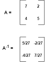
Consider an example where an input x is taken by the function scipy.linalg.inv. This input is the square matrix. It returns y, which is the inverse of the matrix x. Let the matrix be –

Python

# Import the required libraries
from scipy import linalg
import numpy as np

# Initializing the matrix
x = np.array([[7, 2], [4, 5]])

# Finding the inverse of
# matrix x
y = linalg.inv(x)
print(y)

Output:

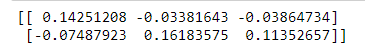
[[ 0.18518519 -0.07407407]
 [-0.14814815  0.25925926]]

Calculating the Pseudo Inverse of a Matrix

To evaluate the (Moore-Penrose) pseudo-inverse of a matrix, scipy.linalg.pinv is used.

Syntax: scipy.linalg.pinv(a , cond , rcond , return_rank , check_finite)

Parameters:

• a: It is the Input Matrix.
• cond, rcond (Optional): It is the cutoff factor for small singular values.
• return_rank (Optional): It returns the effective rank of the matrix if the value is True.
• check_finite (Optional): It checks if the input matrix consists of only finite numbers.

Returns:

• scipy.linalg.pinv returns the pseudo-inverse of the input matrix.

Example: The scipy.linalg.pinv takes a matrix x to be pseudo-inverted. It returns the pseudo-inverse of matrix x and the effective rank of the matrix.

Python

# Import the required libraries
from scipy import linalg
import numpy as np

# Initializing the matrix
x = np.array([[8 , 2] , [3 , 5] , [1 , 3]])

# finding the pseudo inverse of matrix x
y = linalg.pinv(x)
print(y)

Output:

Finding the Determinant of a Matrix

The determinant of a square matrix is a value derived arithmetically from the coefficients of the matrix. In the linalg module, we use the linalg.det() function to find the determinant of a matrix.

Syntax: scipy.linalg.det(a , overwrite_a , check_finite)

Parameters:

• a: It is a square matrix.
• overwrite_a (Optional): It grants permission to overwrite data in a.
• check_finite (Optional): It checks if the input square matrix consists of only finite numbers.

Returns:

• Floating point value

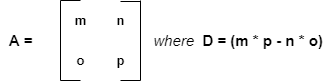
The scipy.linalg.det takes a square matrix A and returns D, the determinant of A. The determinant is a specific property of the linear transformation of a matrix. The determinant of a 2×2 matrix is given by:

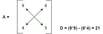
From the above Python code, the determinant is calculated as:

Example:

Python

# Importing the required libraries
from scipy import linalg
import numpy as np

# Initializing the matrix A
A = np.array([[9 , 6] , [4 , 5]])

# Finding the determinant of matrix A
D = linalg.det(A)
print(D)

Output:

21.0

Singular Value Decomposition

The Singular-Value Decomposition is a matrix decomposition method for reducing a matrix to its constituent parts to make specific subsequent matrix calculations simpler. It is calculated using scipy.linalg.svd.

Syntax: scipy.linalg.svd(a , full_matrices , compute_uv , overwrite_a , check_finite , lapack_driver)

Parameters:

• a: The input matrix.
• full_matrices (Optional): If True, the two decomposed unitary matrices of the input matrix are of shape (M, M), (N, N).
• compute_uv (Optional): The default value is True.
• overwrite_a (Optional): It grants permission to overwrite data in a.
• check_finite (Optional): It checks if the input matrix consists of only finite numbers.
• lapack_driver (Optional): It takes either the divide-and-conquer approach (‘gesdd’) or general rectangular approach (‘gesvd’).

The function scipy.linalg.svd takes a matrix M to decompose and returns:

1. A Unitary matrix having left singular vectors as columns.
2. The singular values sorted in non-increasing order.
3. A unitary matrix having right singular vectors as rows.

Example:

Python

# Importing the required libraries
from scipy import linalg
import numpy as np

# Initializing the matrix M
M = np.array([[1 , 5] , [6 , 10]])

# Passing the values to the
# eigen function
x , y , z = linalg.svd(M)
print(x , y , z)

Output:

Eigenvalues and EigenVectors

Let M be an n×n matrix and let X∈Cⁿ be a non-zero vector for which:

MX = λX for some scalar λ.

λ is called an eigenvalue of the matrix M and X is called an eigenvector of M associated with λ, or a λ-eigenvector of M.

Syntax: scipy.linalg.eig(a , b , left , right , overwrite_a , overwrite_b , check_finite , homogeneous_eigvals)

Parameters:

• a: Input matrix.
• b (Optional): It is a right-hand side matrix in a generalized eigenvalue problem.
• left, right (Optional): Whether to compute and return left or right eigenvectors respectively.
• overwrite_a, overwrite_b (Optional): It grants permission to overwrite data in a and b respectively.
• check_finite (Optional): It checks if the input matrix consists of only finite numbers.
• homogeneous_eigvals (Optional): It returns the eigenvalues in homogeneous coordinates if the value is True.

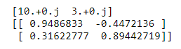
The function scipy.linalg.eig takes a complex or a real matrix M whose eigenvalues and eigenvectors are to be evaluated. It returns the scalar set of eigenvalues for the matrix. It finds the eigenvalues and the right or left eigenvectors of the matrix.

Example:

Python

# Importing the required libraries
from scipy import linalg
import numpy as np

# Initializing the matrix M
M = np.array([[9 , 3] , [2 , 4]])

# Passing the values to the eigen
# function
val , vect = linalg.eig(M)

# Display the Eigen values and Eigen
# vectors
print(val)
print(vect)

Output:

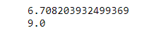
Calculating the norm

To define how close two vectors or matrices are, and to define the convergence of sequences of vectors or matrices, the norm is used. The function scipy.linalg.norm is used to calculate the matrix or vector norm.

Syntax: scipy.linalg.norm(a , ord , axis , keepdims , check_finite)

Parameters:

• a: It is an input array or matrix.
• ord (Optional): It is the order of the norm
• axis (Optional): It denotes the axes.
• keepdims (Optional): If the value is True, the axes which are normed over are left in the output as dimensions with size=1.
• check_finite (Optional): It checks if the input matrix consists of only finite numbers.

Returns:

• scipy.linalg.norm returns the norm of a.

The function scipy.linalg.norm returns one of the seven different matrix norms or one of an infinite number of vector norms. 

1. The L2 norm evaluates the distance of the vector coordinate from the origin of the vector space. It is also known as the Euclidean norm as it is calculated as the Euclidean distance from the origin. The result is a positive distance value.
2. The L1 norm is evaluated as the sum of the absolute vector values. It is an evaluation of the Manhattan distance from the origin of the vector space.

Example:

Python

# Importing the required libraries
from scipy import linalg
import numpy as np

# Initializing the input array
x = np.array([6 , 3])

# Calculating the L2 norm
a = linalg.norm(x)

# Calculating the L1 norm
b = linalg.norm(x , 1)

# Displaying the norm values
print(a)
print(b)

Output:

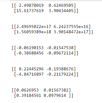
More Matrix Functions

Function Name	Definition
scipy.linalg.sqrtm(A, disp, blocksize)	Finds the square root of the matrix.
scipy.linalg.expm(A)	Computes the matrix exponential using Pade approximation.
scipy.linalg.sinm(A)	Computes the sine of the matrix.
scipy.linalg.cosm(A)	Computes the cosine of the matrix.
scipy.linalg.tanm(A)	Computes the tangent of the matrix.

Example:

Python

# Importing the required libraries
from scipy import linalg
import numpy as np

# Initializing the matrix
x = np.array([[16 , 4] , [100 , 25]])

# Calculate and print the matrix
# square root
r = linalg.sqrtm(x)
print(r)
print("\n")

# Calculate and print the matrix
# exponential
e = linalg.expm(x)
print(e)
print("\n")

# Calculate and print the matrix
# sine
s = linalg.sinm(x)
print(s)
print("\n")

# Calculate and print the matrix
# cosine
c = linalg.cosm(x)
print(c)
print("\n")

# Calculate and print the matrix
# tangent
t = linalg.tanm(x)
print(t)

Output: