Analyzing selling price of used cars using Python
Last Updated :
12 Dec, 2019
Now-a-days, with the technological advancement, Techniques like Machine Learning, etc are being used on a large scale in many organisations. These models usually work with a set of predefined data-points available in the form of datasets. These datasets contain the past/previous information on a specific domain. Organising these datapoints before it is fed to the model is very important. This is where we use Data Analysis. If the data fed to the machine learning model is not well organised, it gives out false or undesired output. This can cause major losses to the organisation. Hence making use of proper data analysis is very important.
About Dataset:
The data that we are going to use in this example is about cars. Specifically containing various information datapoints about the used cars, like their price, color, etc. Here we need to understand that simply collecting data isn’t enough. Raw data isn’t useful. Here data analysis plays a vital role in unlocking the information that we require and to gain new insights into this raw data.
Consider this scenario, our friend, Otis, wants to sell his car. But he doesn’t know how much should he sell his car for! He wants to maximize the profit but he also wants it to be sold for a reasonable price for someone who would want to own it. So here, us, being a data scientist, we can help our friend Otis.
Let’s think like data scientists and clearly define some of his problems: For example, is there data on the prices of other cars and their characteristics? What features of cars affect their prices? Colour? Brand? Does horsepower also affect the selling price, or perhaps, something else?
As a data analyst or data scientist, these are some of the questions we can start thinking about. To answer these questions, we’re going to need some data. But this data is in raw form. Hence we need to analyze it first. The data is available in the form of .csv/.data format with us
To download the file used in this example click here. The file provided is in the .data format. Follow the below process for converting a .data file to .csv file.
Process to convert .data file to .csv:
- open MS Excel
- Go to DATA
- Select From text
- Check box tick on comas(only)
- Save as .csv to your desired location on your pc!
Modules needed:
- pandas: Pandas is an opensource library that allows you to perform data manipulation in Python. Pandas provide an easy way to create, manipulate and wrangle the data.
- numpy: Numpy is the fundamental package for scientific computing with Python.
numpy can be used as an efficient multi-dimensional container of generic data.
- matplotlib: Matplotlib is a Python 2D plotting library which produces publication quality figures in a variety of formats.
- seaborn: Seaborn is a Python data-visualization library that is based on matplotlib. Seaborn provides a high-level interface for drawing attractive and informative statistical graphics.
- scipy: Scipy is a Python-based ecosystem of open-source software for mathematics, science, and engineering.
Steps for installing these packages:
- If you are using anaconda- jupyter/ syder or any other third party softwares to write your python code, make sure to set the path to the “scripts folder” of that software in command prompt of your pc.
- Then type – pip install package-name
Example:
pip install numpy
- Then after the installation is done. (Make sure you are connected to the internet!!) Open your IDE, then import those packages. To import, type – import package name
Example:
import numpy
Steps that are used in the following code (Short description):
- Import the packages
- Set the path to the data file(.csv file)
- Find if there are any null data or NaN data in our file. If any, remove them
- Perform various data cleaning and data visualisation operations on your data. These steps are illustrated beside each line of code in the form of comments for better understanding, as it would be better to see the code side by side than explaining it entirely here, would be meaningless.
- Obtain the result!
Lets start analyzing the data.
Step 1: Import the modules needed.
import pandas as pd
import numpy as np
import matplotlib.pyplot as plt
import seaborn as sns
import scipy as sp
|
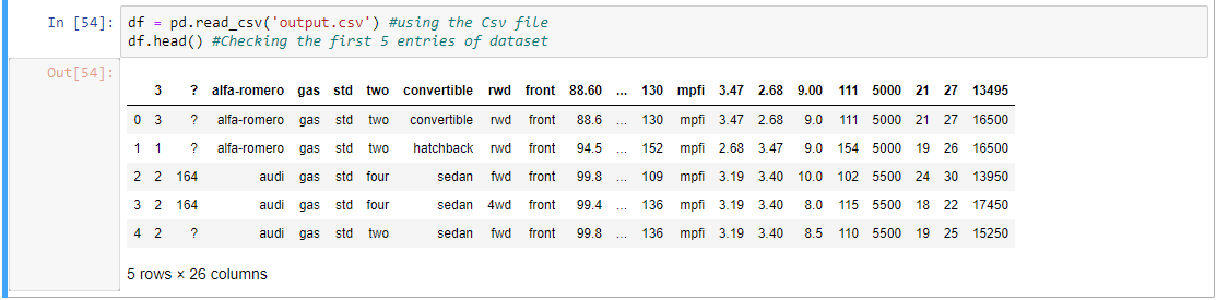
Step 2: Let’s check the first five entries of dataset.
df = pd.read_csv('output.csv')
df.head()
|
Output:
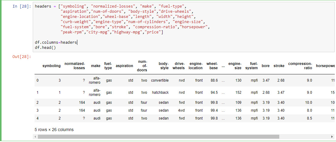
Step 3: Defining headers for our dataset.
headers = ["symboling", "normalized-losses", "make",
"fuel-type", "aspiration","num-of-doors",
"body-style","drive-wheels", "engine-location",
"wheel-base","length", "width","height", "curb-weight",
"engine-type","num-of-cylinders", "engine-size",
"fuel-system","bore","stroke", "compression-ratio",
"horsepower", "peak-rpm","city-mpg","highway-mpg","price"]
df.columns=headers
df.head()
|
Output:
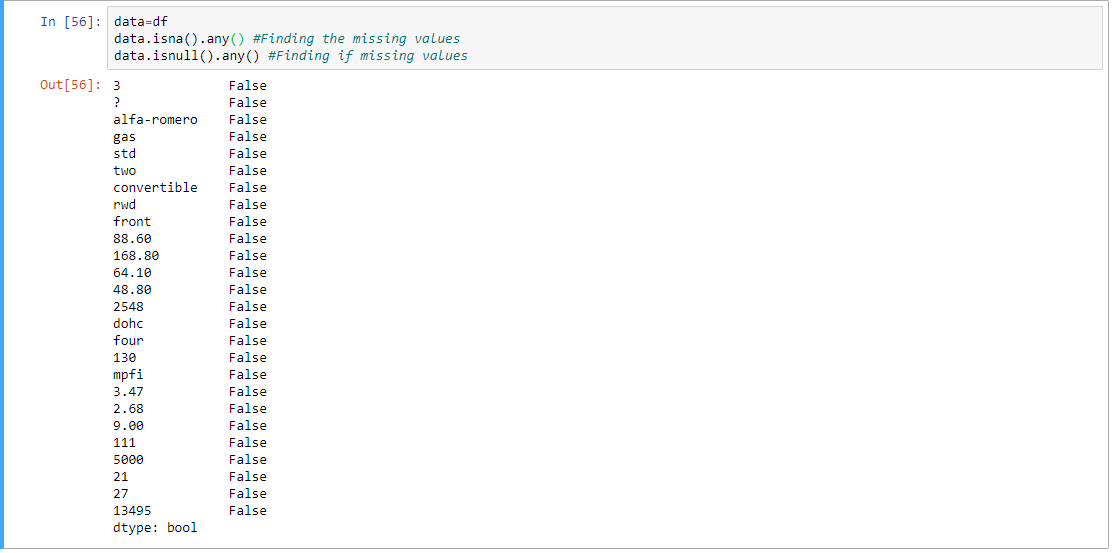
Step 4: Finding the missing value if any.
data = df
data.isna().any()
data.isnull().any()
|
Output:
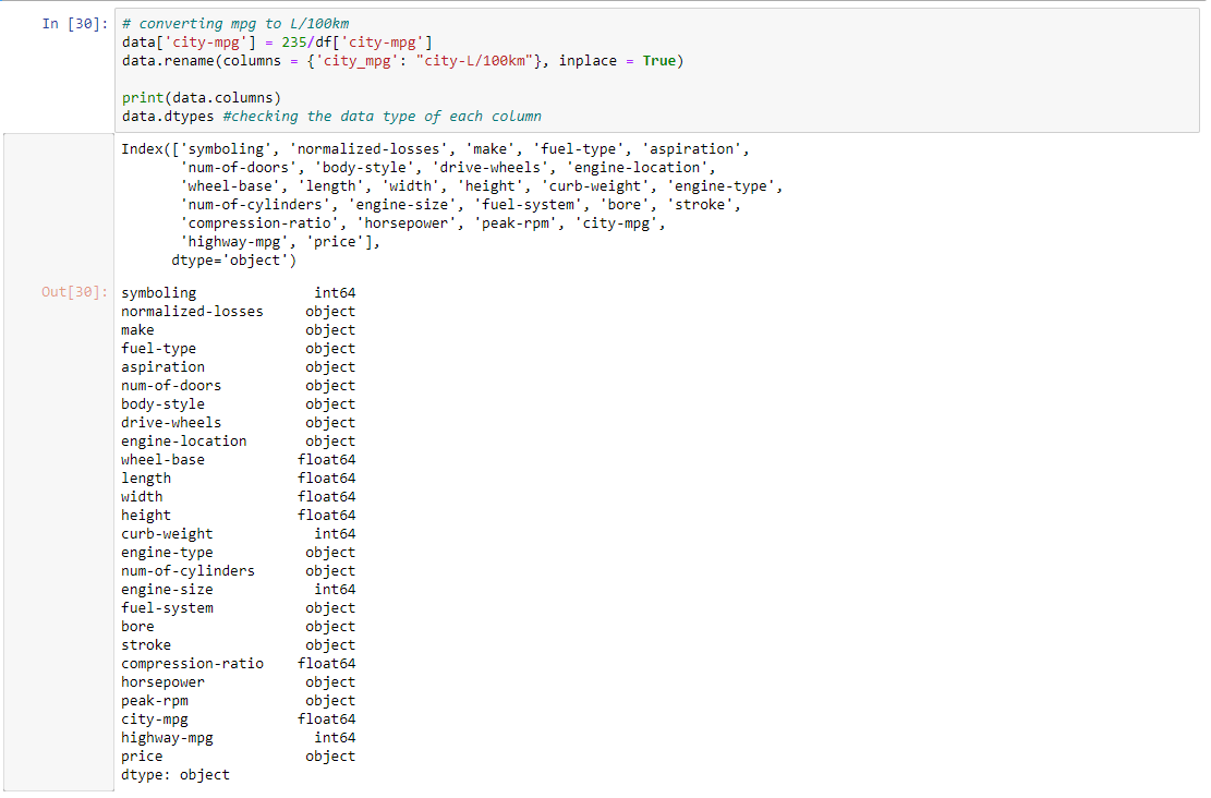
Step 4: Converting mpg to L/100km and checking the data type of each column.
data['city-mpg'] = 235 / df['city-mpg']
data.rename(columns = {'city_mpg': "city-L / 100km"}, inplace = True)
print(data.columns)
data.dtypes
|
Output:
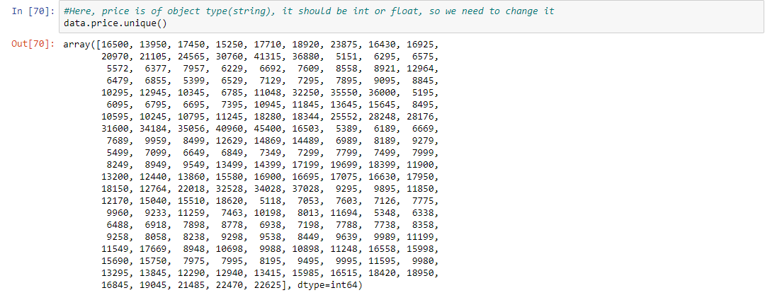
Step 5: Here, price is of object type(string), it should be int or float, so we need to change it
data.price.unique()
data = data[data.price != '?']
data.dtypes
|
Output:

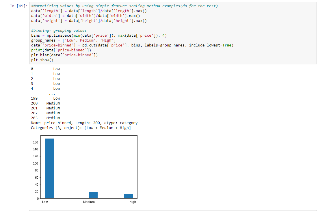
Step 6: Normalizing values by using simple feature scaling method examples(do for the rest) and binning- grouping values
data['length'] = data['length']/data['length'].max()
data['width'] = data['width']/data['width'].max()
data['height'] = data['height']/data['height'].max()
bins = np.linspace(min(data['price']), max(data['price']), 4)
group_names = ['Low', 'Medium', 'High']
data['price-binned'] = pd.cut(data['price'], bins,
labels = group_names,
include_lowest = True)
print(data['price-binned'])
plt.hist(data['price-binned'])
plt.show()
|
Output:
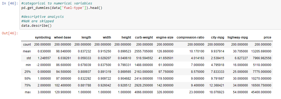
Step 7: Doing descriptive analysis of data categorical to numerical values.
pd.get_dummies(data['fuel-type']).head()
data.describe()
|
Output:
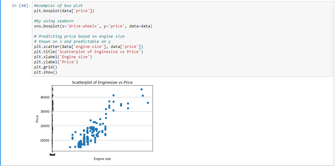
Step 8: Plotting the data according to the price based on engine size.
plt.boxplot(data['price'])
sns.boxplot(x ='drive-wheels', y ='price', data = data)
plt.scatter(data['engine-size'], data['price'])
plt.title('Scatterplot of Enginesize vs Price')
plt.xlabel('Engine size')
plt.ylabel('Price')
plt.grid()
plt.show()
|
Output:
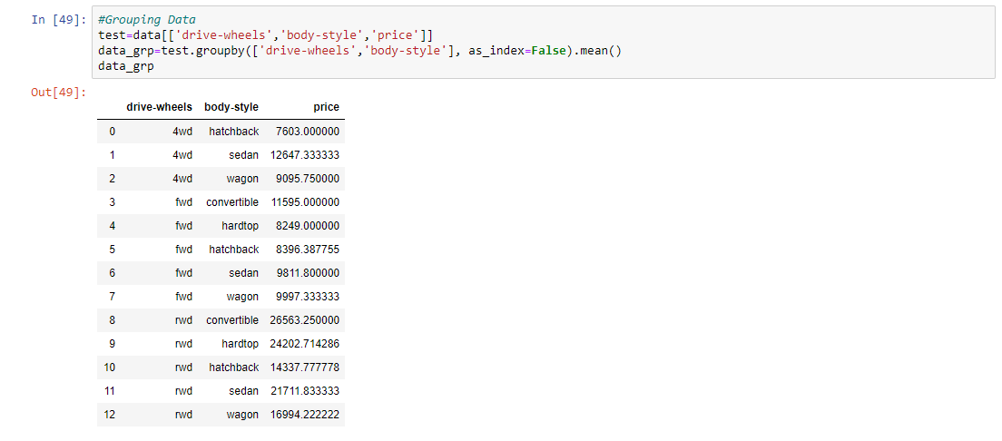
Step 9: Grouping the data according to wheel, body-style and price.
test = data[['drive-wheels', 'body-style', 'price']]
data_grp = test.groupby(['drive-wheels', 'body-style'],
as_index = False).mean()
data_grp
|
Output:
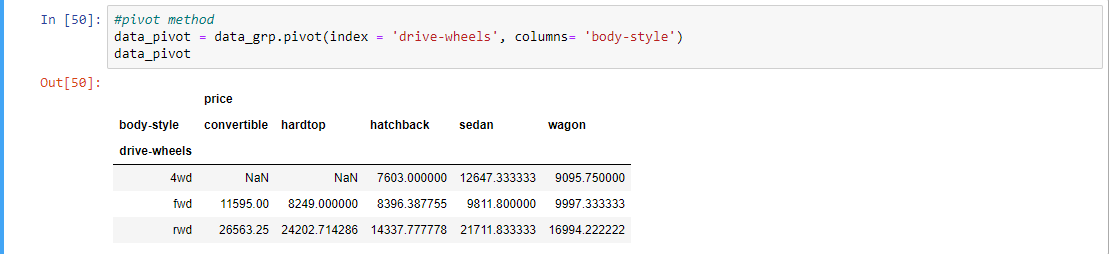
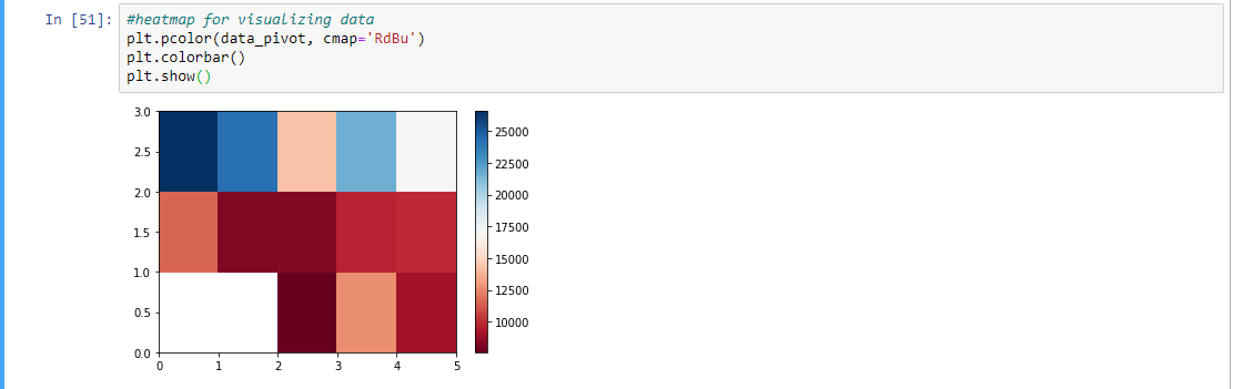
Step 10: Using the pivot method and plotting the heatmap according to the data obtained by pivot method
data_pivot = data_grp.pivot(index = 'drive-wheels',
columns = 'body-style')
data_pivot
plt.pcolor(data_pivot, cmap ='RdBu')
plt.colorbar()
plt.show()
|
Output:
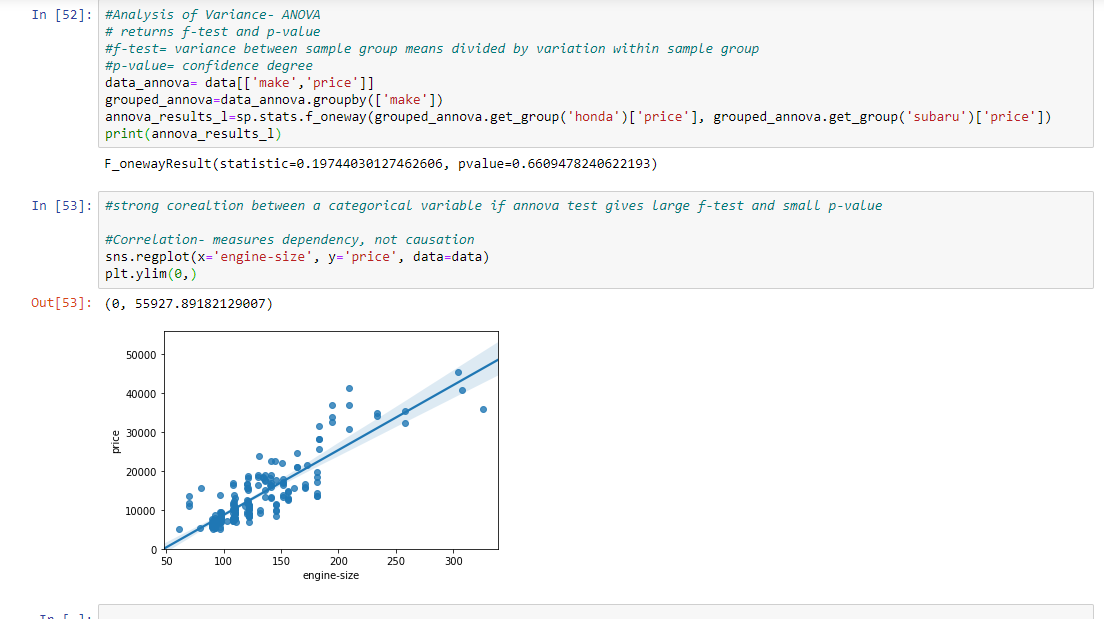
Step 11: Obtaining the final result and showing it in the form of a graph. As the slope is increasing in a positive direction, it is a positive linear relationship.
data_annova = data[['make', 'price']]
grouped_annova = data_annova.groupby(['make'])
annova_results_l = sp.stats.f_oneway(
grouped_annova.get_group('honda')['price'],
grouped_annova.get_group('subaru')['price']
)
print(annova_results_l)
sns.regplot(x ='engine-size', y ='price', data = data)
plt.ylim(0, )
|
Output:
Share your thoughts in the comments
Please Login to comment...