Polynomial Regression is a form of linear regression in which the relationship between the independent variable x and dependent variable y is modelled as an nth-degree polynomial. Polynomial regression fits a nonlinear relationship between the value of x and the corresponding conditional mean of y, denoted E(y | x). In this article, we’ll go in-depth about polynomial regression.
What is a Polynomial Regression?
- There are some relationships that a researcher will hypothesize is curvilinear. Clearly, such types of cases will include a polynomial term.
- Inspection of residuals. If we try to fit a linear model to curved data, a scatter plot of residuals (Y-axis) on the predictor (X-axis) will have patches of many positive residuals in the middle. Hence in such a situation, it is not appropriate.
- An assumption in the usual multiple linear regression analysis is that all the independent variables are independent. In the polynomial regression model, this assumption is not satisfied.
Why Polynomial Regression?
Polynomial regression is a type of regression analysis used in statistics and machine learning when the relationship between the independent variable (input) and the dependent variable (output) is not linear. While simple linear regression models the relationship as a straight line, polynomial regression allows for more flexibility by fitting a polynomial equation to the data.
When the relationship between the variables is better represented by a curve rather than a straight line, polynomial regression can capture the non-linear patterns in the data.
How does a Polynomial Regression work?
If we observe closely then we will realize that to evolve from linear regression to polynomial regression. We are just supposed to add the higher-order terms of the dependent features in the feature space. This is sometimes also known as feature engineering but not exactly.
When the relationship is non-linear, a polynomial regression model introduces higher-degree polynomial terms.
The general form of a polynomial regression equation of degree n is:

where,
- y is the dependent variable.
- x is the independent variable.
 are the coefficients of the polynomial terms.
- n is the degree of the polynomial.
 represents the error term.
The basic goal of regression analysis is to model the expected value of a dependent variable y in terms of the value of an independent variable x. In simple linear regression, we used the following equation –
y = a + bx + e
Here y is a dependent variable, a is the y-intercept, b is the slope and e is the error rate. In many cases, this linear model will not work out For example if we analyze the production of chemical synthesis in terms of the temperature at which the synthesis takes place in such cases we use a quadratic model.
Here,
- y is the dependent variable on x
- a is the y-intercept and e is the error rate.
In general, we can model it for the nth value. 
Since the regression function is linear in terms of unknown variables, hence these models are linear from the point of estimation. Hence through the Least Square technique, response value (y) can be computed.
By including higher-degree terms (quadratic, cubic, etc.), the model can capture the non-linear patterns in the data.
- The choice of the polynomial degree (n) is a crucial aspect of polynomial regression. A higher degree allows the model to fit the training data more closely, but it may also lead to overfitting, especially if the degree is too high. Therefore, the degree should be chosen based on the complexity of the underlying relationship in the data.
- The polynomial regression model is trained to find the coefficients that minimize the difference between the predicted values and the actual values in the training data.
- Once the model is trained, it can be used to make predictions on new, unseen data. The polynomial equation captures the non-linear patterns observed in the training data, allowing the model to generalize to non-linear relationships.
Polynomial Regression Real-Life Example
Let’s consider a real-life example to illustrate the application of polynomial regression. Suppose you are working in the field of finance, and you are analyzing the relationship between the years of experience (in years) an employee has and their corresponding salary (in dollars). You suspect that the relationship might not be linear and that higher degrees of the polynomial might better capture the salary progression over time.
|
|
50,000
|
|
55,000
|
|
65,000
|
|
80,000
|
|
110,000
|
|
150,000
|
|
200,000
|
Now, let’s apply polynomial regression to model the relationship between years of experience and salary. We’ll use a quadratic polynomial (degree 2) for this example.
The quadratic polynomial regression equation is:
Salary= ×Experience+
 ×Experience^2+
Now, to find the coefficients that minimize the difference between the predicted salaries and the actual salaries in the dataset we can use a method of least squares. The objective is to minimize the sum of squared differences between the predicted values and the actual values.
Polynomial Regression implementations using Python
To get the Dataset used for the analysis of Polynomial Regression, click here. Import the important libraries and the dataset we are using to perform Polynomial Regression.
Python libraries make it very easy for us to handle the data and perform typical and complex tasks with a single line of code.
- Pandas – This library helps to load the data frame in a 2D array format and has multiple functions to perform analysis tasks in one go.
- Numpy – Numpy arrays are very fast and can perform large computations in a very short time.
- Matplotlib/Seaborn – This library is used to draw visualizations.
- Sklearn – This module contains multiple libraries having pre-implemented functions to perform tasks from data preprocessing to model development and evaluation.
Python3
import numpy as np
import matplotlib.pyplot as plt
import pandas as pd
datas = pd.read_csv('data.csv')
datas
|
Output:
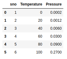
First Five rows of the dataset
Our feature variable that is X will contain the Column between 1st and the target variable that is y will contain the 2nd column.
Python3
X = datas.iloc[:, 1:2].values
y = datas.iloc[:, 2].values
|
Now let’s fit a linear regression model on the data at hand.
Python3
X = datas.iloc[:, 1:2].values
y = datas.iloc[:, 2].values
from sklearn.linear_model import LinearRegression
lin = LinearRegression()
lin.fit(X, y)
|
Fitting the Polynomial Regression model on two components X and y.
Python3
from sklearn.preprocessing import PolynomialFeatures
poly = PolynomialFeatures(degree=4)
X_poly = poly.fit_transform(X)
poly.fit(X_poly, y)
lin2 = LinearRegression()
lin2.fit(X_poly, y)
|
In this step, we are Visualising the Linear Regression results using a scatter plot.
Python3
plt.scatter(X, y, color='blue')
plt.plot(X, lin.predict(X), color='red')
plt.title('Linear Regression')
plt.xlabel('Temperature')
plt.ylabel('Pressure')
plt.show()
|
Output:
.png)
Scatter plot of feature and the target variable.
Visualize the Polynomial Regression results using a scatter plot.
Python3
plt.scatter(X, y, color='blue')
plt.plot(X, lin2.predict(poly.fit_transform(X)),
color='red')
plt.title('Polynomial Regression')
plt.xlabel('Temperature')
plt.ylabel('Pressure')
plt.show()
|
Output:
.png)
Implementation of Polynomial Regression
Predict new results with both Linear and Polynomial Regression. Note that the input variable must be in a Numpy 2D array.
Python3
pred = 110.0
predarray = np.array([[pred]])
lin.predict(predarray)
|
Output:
array([0.20675333])
Python3
pred2 = 110.0
pred2array = np.array([[pred2]])
lin2.predict(poly.fit_transform(pred2array))
|
Output:
array([0.43295877])
Overfitting Vs Under-fitting
While dealing with the polynomial regression one thing that we face is the problem of overfitting this happens because while we increase the order of the polynomial regression to achieve better and better performance model gets overfit on the data and does not perform on the new data points.
Due to this reason only while using the polynomial regression, do we try to penalize the weights of the model to regularize the effect of the overfitting problem. Regularization techniques like Lasso regression and Ridge regression methodologies are used whenever we deal with a situation in which the model may overfit the data at hand.
Bias Vs Variance Tradeoff
This technique is the generalization of the approach that is used to avoid the problem of overfitting and underfitting. Here as well this technique helps us to avoid the problem of overfitting by helping us select the appropriate value for the degree of the polynomial we are trying to fit our data on. For example, this is achieved when after increasing the degree of polynomial after a certain level the gap between the training and the validation metrics starts increasing.
Application of Polynomial Regression
The reason behind the vast use cases of the polynomial regression is that approximately all of the real-world data is non-linear in nature and hence when we fit a non-linear model on the data or a curvilinear regression line then the results that we obtain are far better than what we can achieve with the standard linear regression. Some of the use cases of the Polynomial regression are as stated below:
- The growth rate of tissues.
- Progression of disease epidemics
- Distribution of carbon isotopes in lake sediments
Advantages & Disadvantages of using Polynomial Regression
Advantages of using Polynomial Regression
- A broad range of functions can be fit under it.
- Polynomial basically fits a wide range of curvatures.
- Polynomial provides the best approximation of the relationship between dependent and independent variables.
Disadvantages of using Polynomial Regression
- These are too sensitive to outliers.
- The presence of one or two outliers in the data can seriously affect the results of nonlinear analysis.
- In addition, there are unfortunately fewer model validation tools for the detection of outliers in nonlinear regression than there are for linear regression.
Conclusion
Polynomial regression, a versatile tool, finds applications in diverse domains. While addressing non-linear relationships, it requires careful consideration of overfitting and model complexity.
Frequently Asked Questions(FAQs)
1.What is a real life example of polynomial regression?
Predicting car fuel efficiency based on engine power—capturing non-linear patterns in the relationship.
2.What is polynomial regression pipeline?
A sequence of data processing steps, like polynomial feature creation and linear regression, streamlining polynomial regression modeling.
3.What is polynomial regression Excel?
Excel can perform polynomial regression using the “LINEST” function or the “Trendline” feature in a scatter plot.
4.What is polynomial regression with example?
Modeling stock prices over time using a quadratic polynomial to capture potential non-linear trends in the data.
5.What is the purpose of polynomial regression?
Captures non-linear relationships in data, providing a flexible model for complex patterns beyond linear regression’s scope.
Share your thoughts in the comments
Please Login to comment...