Polynomial Regression for Non-Linear Data – ML
Last Updated :
03 Jun, 2020
Non-linear data is usually encountered in daily life. Consider some of the equations of motion as studied in physics.
- Projectile Motion: The height of a projectile is calculated as h = -½ gt2 +ut +ho
- Equation of motion under free fall: The distance travelled by an object after falling freely under gravity for ‘t’ seconds is ½ g t2.
- Distance travelled by a uniformly accelerated body: The distance can be calculated as ut + ½at2
where,
g = acceleration due to gravity
u = initial velocity
ho = initial height
a = acceleration
In addition to these examples, Non-linear trends are also observed in the growth rate of tissues, the progress of disease epidemic, black body radiation, the motion of the pendulum etc. These examples clearly indicate that we cannot always have a linear relationship between the independent and dependent attributes. Hence, linear regression is a poor choice for dealing with such nonlinear situations. This is where Polynomial Regression comes to our rescue!!
Polynomial Regression is a powerful technique to encounter the situations where a quadratic, cubic or a higher degree nonlinear relationship exists. The underlying concept in polynomial regression is to add powers of each independent attribute as new attributes and then train a linear model on this expanded collection of features.
Let us illustrate the use of Polynomial Regression with an example. Consider a situation where the dependent variable y varies with respect to an independent variable x following a relation
y = 13x2 + 2x + 7
.
We shall use Scikit-Learn’s PolynomialFeatures class for the implementation.
Step1: Import the libraries and generate a random dataset.
import numpy as np
import matplotlib.pyplot as plt
from sklearn.linear_model import LinearRegression
from sklearn.preprocessing import PolynomialFeatures
from sklearn.metrics import mean_squared_error, r2_score
x = np.array(7 * np.random.rand(100, 1) - 3)
x1 = x.reshape(-1, 1)
y = 13 * x*x + 2 * x + 7
|
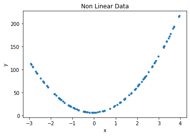
Step2: Plot the data points.
plt.scatter(x, y, s = 10)
plt.xlabel('x')
plt.ylabel('y')
plt.title('Non Linear Data')
|
Step3: First try to fit the data with a linear model.
regression_model = LinearRegression()
regression_model.fit(x1, y)
print('Slope of the line is', regression_model.coef_)
print('Intercept value is', regression_model.intercept_)
y_predicted = regression_model.predict(x1)
|
Output:
Slope of the line is [[14.87780012]]
Intercept value is [58.31165769]
Step 4: Plot the data points and the linear line.
plt.scatter(x, y, s = 10)
plt.xlabel("$x$", fontsize = 18)
plt.ylabel("$y$", rotation = 0, fontsize = 18)
plt.title("data points")
plt.plot(x, y_predicted, color ='g')
|
Output:
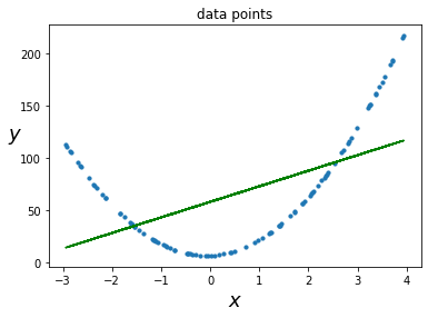
Equation of the linear model is y = 14.87x + 58.31
Step 5: Calculate the performance of the model in terms of mean square error, root mean square error and r2 score.
mse = mean_squared_error(y, y_predicted)
rmse = np.sqrt(mean_squared_error(y, y_predicted))
r2 = r2_score(y, y_predicted)
print('MSE of Linear model', mse)
print('R2 score of Linear model: ', r2)
|
Output:
MSE of Linear model 2144.8229656677095
R2 score of Linear model:  0.3019970606151057
The performance of the linear model is not satisfactory. Let’s try Polynomial Regression with degree 2
Step 6: For improving the performance, we need to make the model a bit complex. So, lets fit a polynomial of degree 2 and proceed with linear regression.
poly_features = PolynomialFeatures(degree = 2, include_bias = False)
x_poly = poly_features.fit_transform(x1)
x[3]
|
Output:
Out[]:array([-2.84314447])
Output:
Out[]:array([-2.84314447, 8.08347046])
In addition to column x, one more column has been introduced which is the square of actual data. Now we proceed with simple Linear Regression
lin_reg = LinearRegression()
lin_reg.fit(x_poly, y)
print('Coefficients of x are', lin_reg.coef_)
print('Intercept is', lin_reg.intercept_)
|
Output:
Coefficients of x are [[ 2. 13.]]
Intercept is [7.]
This is the desired equation 13x2 + 2x + 7
Step 7: Plot the quadratic equation obtained.
x_new = np.linspace(-3, 4, 100).reshape(100, 1)
x_new_poly = poly_features.transform(x_new)
y_new = lin_reg.predict(x_new_poly)
plt.plot(x, y, "b.")
plt.plot(x_new, y_new, "r-", linewidth = 2, label ="Predictions")
plt.xlabel("$x_1$", fontsize = 18)
plt.ylabel("$y$", rotation = 0, fontsize = 18)
plt.legend(loc ="upper left", fontsize = 14)
plt.title("Quadratic_predictions_plot")
plt.show()
|
Output: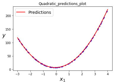
Step 8: Calculate the performance of the model obtained by Polynomial Regression.
y_deg2 = lin_reg.predict(x_poly)
mse_deg2 = mean_squared_error(y, y_deg2)
r2_deg2 = r2_score(y, y_deg2)
print('MSE of Polyregression model', mse_deg2)
print('R2 score of Linear model: ', r2_deg2)
|
Output:
MSE of Polyregression model 7.668437973562934e-28
R2 score of Linear model:  1.0
The performance of polynomial regression model is far better than linear regression model for the given quadratic equation.
Important Facts: PolynomialFeatures (degree = d) transforms an array containing n features into an array containing (n + d)! / d! n! features.
Conclusion: Polynomial Regression is an effective way to deal with nonlinear data as it can find relationships between features which plain Linear Regression model struggles to do.
Share your thoughts in the comments
Please Login to comment...