Artificial Intelligence is the study of building agents that act rationally. Most of the time, these agents perform some kind of search algorithm in the background in order to achieve their tasks.
- A search problem consists of:
- A State Space. Set of all possible states where you can be.
- A Start State. The state from where the search begins.
- A Goal State. A function that looks at the current state returns whether or not it is the goal state.
- The Solution to a search problem is a sequence of actions, called the plan that transforms the start state to the goal state.
- This plan is achieved through search algorithms.
Types of search algorithms:
There are far too many powerful search algorithms out there to fit in a single article. Instead, this article will discuss six of the fundamental search algorithms, divided into two categories, as shown below.
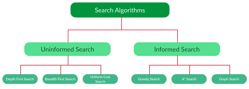
Note that there is much more to search algorithms than the chart I have provided above. However, this article will mostly stick to the above chart, exploring the algorithms given there.
Uninformed Search Algorithms:
The search algorithms in this section have no additional information on the goal node other than the one provided in the problem definition. The plans to reach the goal state from the start state differ only by the order and/or length of actions. Uninformed search is also called Blind search. These algorithms can only generate the successors and differentiate between the goal state and non goal state.
The following uninformed search algorithms are discussed in this section.
- Depth First Search
- Breadth First Search
- Uniform Cost Search
Each of these algorithms will have:
- A problem graph, containing the start node S and the goal node G.
- A strategy, describing the manner in which the graph will be traversed to get to G.
- A fringe, which is a data structure used to store all the possible states (nodes) that you can go from the current states.
- A tree, that results while traversing to the goal node.
- A solution plan, which the sequence of nodes from S to G.
Depth-first search (DFS) is an algorithm for traversing or searching tree or graph data structures. The algorithm starts at the root node (selecting some arbitrary node as the root node in the case of a graph) and explores as far as possible along each branch before backtracking. It uses last in- first-out strategy and hence it is implemented using a stack.
Example:
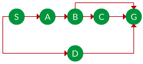
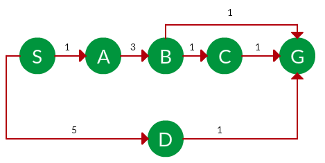
Question. Which solution would DFS find to move from node S to node G if run on the graph below?
Solution. The equivalent search tree for the above graph is as follows. As DFS traverses the tree “deepest node first”, it would always pick the deeper branch until it reaches the solution (or it runs out of nodes, and goes to the next branch). The traversal is shown in blue arrows.
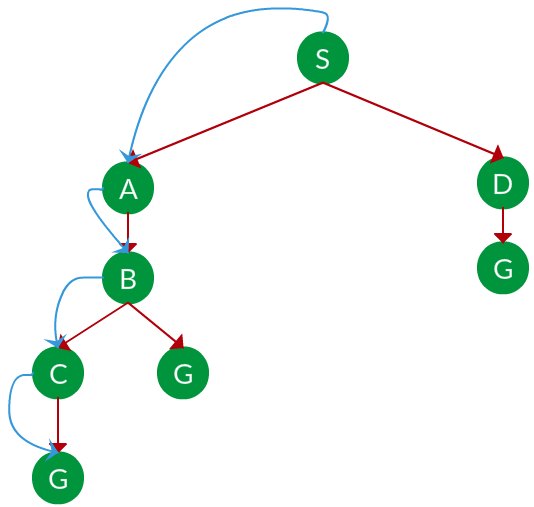
Path: S -> A -> B -> C -> G
 = the depth of the search tree = the number of levels of the search tree.
 = number of nodes in level
  .
.
Time complexity: Equivalent to the number of nodes traversed in DFS. 
Space complexity: Equivalent to how large can the fringe get. 
Completeness: DFS is complete if the search tree is finite, meaning for a given finite search tree, DFS will come up with a solution if it exists.
Optimality: DFS is not optimal, meaning the number of steps in reaching the solution, or the cost spent in reaching it is high.
Breadth-first search (BFS) is an algorithm for traversing or searching tree or graph data structures. It starts at the tree root (or some arbitrary node of a graph, sometimes referred to as a ‘search key’), and explores all of the neighbor nodes at the present depth prior to moving on to the nodes at the next depth level. It is implemented using a queue.
Example:
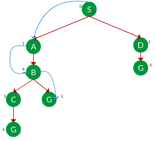
Question. Which solution would BFS find to move from node S to node G if run on the graph below?
Solution. The equivalent search tree for the above graph is as follows. As BFS traverses the tree “shallowest node first”, it would always pick the shallower branch until it reaches the solution (or it runs out of nodes, and goes to the next branch). The traversal is shown in blue arrows.
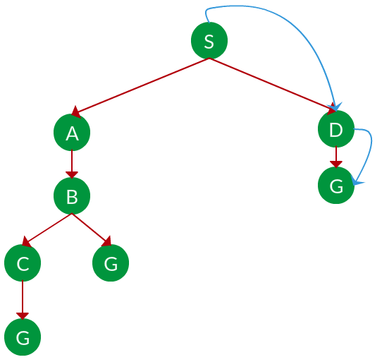
Path: S -> D -> G
 = the depth of the shallowest solution.
= number of nodes in level .
Time complexity: Equivalent to the number of nodes traversed in BFS until the shallowest solution. 
Space complexity: Equivalent to how large can the fringe get. 
Completeness: BFS is complete, meaning for a given search tree, BFS will come up with a solution if it exists.
Optimality: BFS is optimal as long as the costs of all edges are equal.
Uniform Cost Search:
UCS is different from BFS and DFS because here the costs come into play. In other words, traversing via different edges might not have the same cost. The goal is to find a path where the cumulative sum of costs is the least.
Cost of a node is defined as:
  cost(node) = cumulative cost of all nodes from root
  cost(root) = 0
Example:
Question. Which solution would UCS find to move from node S to node G if run on the graph below?
Solution. The equivalent search tree for the above graph is as follows. The cost of each node is the cumulative cost of reaching that node from the root. Based on the UCS strategy, the path with the least cumulative cost is chosen. Note that due to the many options in the fringe, the algorithm explores most of them so long as their cost is low, and discards them when a lower-cost path is found; these discarded traversals are not shown below. The actual traversal is shown in blue.
Path: S -> A -> B -> G
Cost: 5
Let  = cost of solution.
 = arcs cost.
Then  effective depth
Time complexity:  , Space complexity:
Advantages:
- UCS is complete only if states are finite and there should be no loop with zero weight.
- UCS is optimal only if there is no negative cost.
Disadvantages:
- Explores options in every “direction”.
- No information on goal location.
Informed Search Algorithms:
Here, the algorithms have information on the goal state, which helps in more efficient searching. This information is obtained by something called a heuristic.
In this section, we will discuss the following search algorithms.
- Greedy Search
- A* Tree Search
- A* Graph Search
Search Heuristics: In an informed search, a heuristic is a function that estimates how close a state is to the goal state. For example – Manhattan distance, Euclidean distance, etc. (Lesser the distance, closer the goal.) Different heuristics are used in different informed algorithms discussed below.
Greedy Search:
In greedy search, we expand the node closest to the goal node. The “closeness” is estimated by a heuristic h(x).
Heuristic: A heuristic h is defined as-
h(x) = Estimate of distance of node x from the goal node.
Lower the value of h(x), closer is the node from the goal.
Strategy: Expand the node closest to the goal state, i.e. expand the node with a lower h value.
Example:
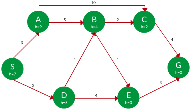
Question. Find the path from S to G using greedy search. The heuristic values h of each node below the name of the node.
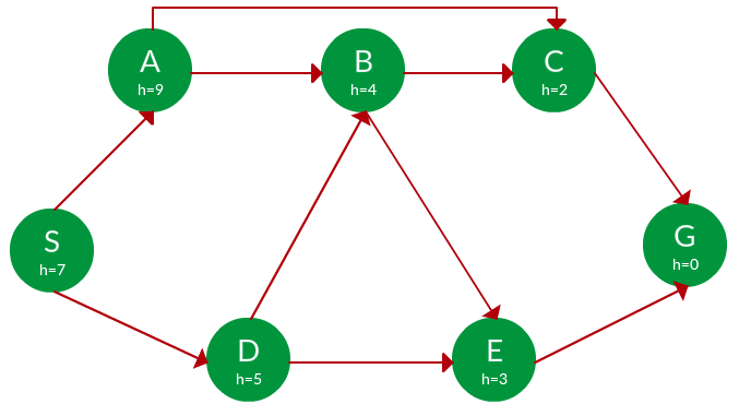
Solution. Starting from S, we can traverse to A(h=9) or D(h=5). We choose D, as it has the lower heuristic cost. Now from D, we can move to B(h=4) or E(h=3). We choose E with a lower heuristic cost. Finally, from E, we go to G(h=0). This entire traversal is shown in the search tree below, in blue.
Path: S -> D -> E -> G
Advantage: Works well with informed search problems, with fewer steps to reach a goal.
Disadvantage: Can turn into unguided DFS in the worst case.
A* Tree Search:
A* Tree Search, or simply known as A* Search, combines the strengths of uniform-cost search and greedy search. In this search, the heuristic is the summation of the cost in UCS, denoted by g(x), and the cost in the greedy search, denoted by h(x). The summed cost is denoted by f(x).
Heuristic: The following points should be noted wrt heuristics in A* search. 
- Here, h(x) is called the forward cost and is an estimate of the distance of the current node from the goal node.
- And, g(x) is called the backward cost and is the cumulative cost of a node from the root node.
- A* search is optimal only when for all nodes, the forward cost for a node h(x) underestimates the actual cost h*(x) to reach the goal. This property of A* heuristic is called admissibility.
Admissibility:

Strategy: Choose the node with the lowest f(x) value.
Example:
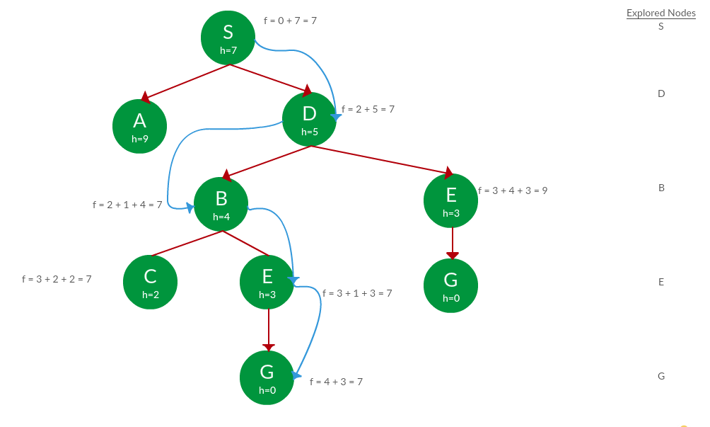
Question. Find the path to reach from S to G using A* search.
Solution. Starting from S, the algorithm computes g(x) + h(x) for all nodes in the fringe at each step, choosing the node with the lowest sum. The entire work is shown in the table below.
Note that in the fourth set of iterations, we get two paths with equal summed cost f(x), so we expand them both in the next set. The path with a lower cost on further expansion is the chosen path.
| Path | h(x) | g(x) | f(x) |
|---|
| S | 7 | 0 | 7 |
|---|
| | | | |
|---|
| S -> A | 9 | 3 | 12 |
|---|
| S -> D ✔ | 5 | 2 | 7 |
|---|
| | | | |
|---|
| S -> D -> B ✔ | 4 | 2 + 1 = 3 | 7 |
|---|
| S -> D -> E | 3 | 2 + 4 = 6 | 9 |
|---|
| | | | |
|---|
| S -> D -> B -> C ✔ | 2 | 3 + 2 = 5 | 7 |
|---|
| S -> D -> B -> E ✔ | 3 | 3 + 1 = 4 | 7 |
|---|
| | | | |
|---|
| S -> D -> B -> C -> G | 0 | 5 + 4 = 9 | 9 |
|---|
| S -> D -> B -> E -> G ✔ | 0 | 4 + 3 = 7 | 7 |
|---|
Path: S -> D -> B -> E -> G
Cost: 7
- A* tree search works well, except that it takes time re-exploring the branches it has already explored. In other words, if the same node has expanded twice in different branches of the search tree, A* search might explore both of those branches, thus wasting time
- A* Graph Search, or simply Graph Search, removes this limitation by adding this rule: do not expand the same node more than once.
- Heuristic. Graph search is optimal only when the forward cost between two successive nodes A and B, given by h(A) – h (B), is less than or equal to the backward cost between those two nodes g(A -> B). This property of the graph search heuristic is called consistency.
Consistency:

Example:
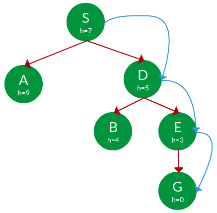
Question. Use graph searches to find paths from S to G in the following graph.
the Solution. We solve this question pretty much the same way we solved last question, but in this case, we keep a track of nodes explored so that we don’t re-explore them.
Path: S -> D -> B -> E -> G
Cost: 7
Share your thoughts in the comments
Please Login to comment...