How to proceed from Simple to Multiple and Polynomial Regression in R

Regression analysis allows us to understand how one or more independent variables relate to a dependent variable. Simple linear regression, which explores the relationship between two variables. Multiple linear regression extends this to include several predictors simultaneously. Finally, polynomial regression introduces flexibility by accommodating non-linear relationships in the R Programming Language.

Simple Regression

Simple regression, also known as simple linear regression, is a statistical method used to model the relationship between two variables. The relationship between the variables is assumed to be linear, meaning that a straight line can adequately describe the association between them.

Y = β₀ + β₁X + ε

Where:

• Y is the dependent variable.
• X is the independent variable.
• β₀ is the intercept (the value of Y when X is zero).
• β₁ is the slope (the change in Y corresponding to a one-unit change in X).
• ε is the error term, representing the difference between the observed and predicted values of Y.

The goal of simple regression is to estimate the values of β₀ and β₁ that minimize the sum of squared differences between the observed and predicted values of Y. Once the model is fitted, we can use it to make predictions about the dependent variable based on new values of the independent variable.

Start with simple linear regression to understand the relationship between one independent variable and one dependent variable.

• Use the lm() function in R to fit a simple linear regression model.

R

# Sample data
x <- c(1, 2, 3, 4, 5)
y <- c(2, 4, 5, 4, 6)

# Fit simple linear regression model
model <- lm(y ~ x)

# Summary of the model
summary(model)

Output:

Call:
lm(formula = y ~ x)

Residuals:
   1    2    3    4    5 
-0.6  0.6  0.8 -1.0  0.2 

Coefficients:
            Estimate Std. Error t value Pr(>|t|)  
(Intercept)   1.8000     0.9381   1.919   0.1508  
x             0.8000     0.2828   2.828   0.0663 .
---
Signif. codes:  0 ‘***’ 0.001 ‘**’ 0.01 ‘*’ 0.05 ‘.’ 0.1 ‘ ’ 1

Residual standard error: 0.8944 on 3 degrees of freedom
Multiple R-squared:  0.7273,    Adjusted R-squared:  0.6364 
F-statistic:     8 on 1 and 3 DF,  p-value: 0.06628

The “Call” section shows the formula used for the regression. The “Residuals” section displays the differences between the observed and predicted values. The “Coefficients” section provides estimates for the intercept and slope of the regression line, along with their standard errors and statistical significance. The “Residual standard error” indicates the average distance of data points from the regression line. The “Multiple R-squared” and “Adjusted R-squared” values measure the goodness of fit of the regression model. The “F-statistic” tests the overall significance of the model, with its associated p-value.

Multiple Regression

Multiple regression, also known as multiple linear regression, is a statistical technique used to model the relationship between a dependent variable and two or more independent variables. In multiple regression, we need to understand how changes in multiple predictors are associated with changes in the dependent variable.

y=β₀ ​ +β_{1 ​} x_{1 ​} +β₂ ​x₂ ​ + … +β_n ​x_{n ​}+ ε

Where:

• y is the dependent variable.
• x₁, x₂,…, x_n are the independent variables (predictors).
• β₀ is the intercept (the value of y when all predictors are zero).
• β₁, β₂,…, β_n are the coefficients representing the effect of each predictor on y.
• ε is the error term, representing the difference between the observed and predicted values of y.

Multiple regression is to estimate the values of the coefficients β1, β2,…, βn that minimize the sum of squared differences between the observed and predicted values of y. Once the model is fitted, we can use it to make predictions about the dependent variable based on new values of the independent variables.

Transition to multiple linear regression when you have more than one independent variable.

• Use the lm() function similarly, but include multiple predictors in the formula.

R

# Sample data
x1 <- c(1, 2, 3, 4, 5)
x2 <- c(2, 3, 4, 5, 6)
y <- c(2, 4, 5, 4, 6)

# Fit multiple linear regression model
model <- lm(y ~ x1 + x2)

# Summary of the model
summary(model)

Output:

Call:
lm(formula = y ~ x1 + x2)

Residuals:
   1    2    3    4    5 
-0.6  0.6  0.8 -1.0  0.2 

Coefficients: (1 not defined because of singularities)
            Estimate Std. Error t value Pr(>|t|)  
(Intercept)   1.8000     0.9381   1.919   0.1508  
x1            0.8000     0.2828   2.828   0.0663 .
x2                NA         NA      NA       NA  
---
Signif. codes:  0 ‘***’ 0.001 ‘**’ 0.01 ‘*’ 0.05 ‘.’ 0.1 ‘ ’ 1

Residual standard error: 0.8944 on 3 degrees of freedom
Multiple R-squared:  0.7273,    Adjusted R-squared:  0.6364 
F-statistic:     8 on 1 and 3 DF,  p-value: 0.06628

Here, output represents the results of a multiple linear regression model fitted to data with two independent variables (x1 and x2) and one dependent variable (y).

Polynomial Regression

Polynomial regression is a type of regression analysis where the relationship between the independent variable(s) and the dependent variable is modeled as an nth-degree polynomial. Unlike simple or multiple linear regression, which assume a linear relationship between variables, polynomial regression can capture non-linear relationships between variables.

y=β₀ ​+β₁ ​x + β₂ x² +…+ β_{n ​} xⁿ + ε

Where:

• y is the dependent variable.
• x is the independent variable.
• x², x³, …, xⁿ are the polynomial terms, representing the square, cube, and higher-order terms of x.
• β₀ , β₁ ​, … , β_n are the coefficients, representing the effect of each polynomial term on y.
• ε is the error term, representing the difference between the observed and predicted values of y.

Polynomial regression extends linear regression by considering polynomial terms of the independent variable.

• Use the poly() function in R to generate polynomial terms.
• Fit the model using lm() with polynomial terms included.

R

# Sample data
x <- c(1, 2, 3, 4, 5)
y <- c(2, 4, 5, 4, 6)

# Fit polynomial regression model (e.g., quadratic)
model <- lm(y ~ poly(x, degree = 2))

# Summary of the model
summary(model)

Output:

Call:
lm(formula = y ~ poly(x, degree = 2))

Residuals:
      1       2       3       4       5 
-0.3143  0.4571  0.5143 -1.1429  0.4857 

Coefficients:
                     Estimate Std. Error t value Pr(>|t|)  
(Intercept)            4.2000     0.4598   9.134   0.0118 *
poly(x, degree = 2)1   2.5298     1.0282   2.460   0.1330  
poly(x, degree = 2)2  -0.5345     1.0282  -0.520   0.6550  
---
Signif. codes:  0 ‘***’ 0.001 ‘**’ 0.01 ‘*’ 0.05 ‘.’ 0.1 ‘ ’ 1

Residual standard error: 1.028 on 2 degrees of freedom
Multiple R-squared:  0.7597,    Adjusted R-squared:  0.5195 
F-statistic: 3.162 on 2 and 2 DF,  p-value: 0.2403

This output is from a polynomial regression model fitted to data with one independent variable (x) and one dependent variable (y).

• Residuals: Differences between observed and predicted values of y.
• Coefficients: Estimates of intercept and polynomial terms (poly(x, degree = 2)).
  • Estimate: Coefficient values.
  • Std. Error: Standard errors.
  • t value: T-statistics for significance.
  • Pr(>|t|): P-values indicating significance.
• Model Fit:
  • Residual standard error: Standard deviation of residuals.
  • Multiple R-squared: Approximately 75.97% of variance explained.
  • Adjusted R-squared: Adjusted for predictors.
  • F-statistic: Tests overall model significance.

Proceed from Simple to Multiple and Polynomial Regression in R

Transitioning from simple linear regression to multiple regression and then polynomial regression in R can be done step by step.

R

# Sample data for demonstration
# for reproducibility
set.seed(123)  
x <- 1:20
y <- 3*x + rnorm(20, mean = 0, sd = 5)  # simple linear relationship with noise
z <- x^2 + rnorm(20, mean = 0, sd = 10)  # quadratic relationship with noise

# Create a dataframe with the variables
data <- data.frame(x, y, z)

# Simple Linear Regression
# Fit a simple linear regression model
lm_simple <- lm(y ~ x, data = data)

# Multiple Linear Regression
# Fit a multiple linear regression model with both x and z as predictors
lm_multiple <- lm(y ~ x + z, data = data)

# Polynomial Regression
# Fit a polynomial regression model (quadratic)
lm_polynomial <- lm(y ~ poly(x, degree = 2), data = data)

# Summary of models
summary(lm_simple)
summary(lm_multiple)
summary(lm_polynomial)

# Plotting the results
par(mfrow = c(1, 3))  # Arrange plots in one row with three columns

# Plot for Simple Linear Regression
plot(x, y, main = "Simple Linear Regression", xlab = "x", ylab = "y")
abline(lm_simple, col = "red")

# Plot for Multiple Linear Regression
plot(x, y, main = "Multiple Linear Regression", xlab = "x", ylab = "y")
points(x, z, col = "blue")  # Adding z to the plot
legend("topleft", legend = c("y", "z"), col = c("black", "blue"), pch = 1)

# Plot for Polynomial Regression
plot(x, y, main = "Polynomial Regression", xlab = "x", ylab = "y")
curve(predict(lm_polynomial, newdata = data.frame(x = x)), add = TRUE, col = "red")

par(mfrow = c(1, 1))  # Reset the plotting layout

Output:

summary(lm_simple)

Call:
lm(formula = y ~ x, data = data)

Residuals:
    Min      1Q  Median      3Q     Max 
-9.9395 -3.0140 -0.1884  2.5971  8.6677 

Coefficients:
            Estimate Std. Error t value Pr(>|t|)    
(Intercept)   1.5505     2.3100   0.671    0.511    
x             2.9198     0.1928  15.141  1.1e-11 ***
---
Signif. codes:  0 ‘***’ 0.001 ‘**’ 0.01 ‘*’ 0.05 ‘.’ 0.1 ‘ ’ 1

Residual standard error: 4.973 on 18 degrees of freedom
Multiple R-squared:  0.9272,    Adjusted R-squared:  0.9232 
F-statistic: 229.3 on 1 and 18 DF,  p-value: 1.102e-11

summary(lm_multiple)

Call:
lm(formula = y ~ x + z, data = data)

Residuals:
    Min      1Q  Median      3Q     Max 
-9.4663 -2.9935 -0.4392  3.0135  8.6904 

Coefficients:
            Estimate Std. Error t value Pr(>|t|)   
(Intercept) -0.65546    4.22722  -0.155  0.87860   
x            3.48640    0.92366   3.775  0.00151 **
z           -0.02618    0.04170  -0.628  0.53850   
---
Signif. codes:  0 ‘***’ 0.001 ‘**’ 0.01 ‘*’ 0.05 ‘.’ 0.1 ‘ ’ 1

Residual standard error: 5.059 on 17 degrees of freedom
Multiple R-squared:  0.9289,    Adjusted R-squared:  0.9205 
F-statistic:   111 on 2 and 17 DF,  p-value: 1.751e-10

summary(lm_polynomial)

Call:
lm(formula = y ~ poly(x, degree = 2), data = data)

Residuals:
   Min     1Q Median     3Q    Max 
-9.482 -3.201 -0.427  2.925  8.608 

Coefficients:
                     Estimate Std. Error t value Pr(>|t|)    
(Intercept)            32.208      1.135  28.372 9.27e-16 ***
poly(x, degree = 2)1   75.294      5.077  14.831 3.71e-11 ***
poly(x, degree = 2)2   -2.635      5.077  -0.519     0.61    
---
Signif. codes:  0 ‘***’ 0.001 ‘**’ 0.01 ‘*’ 0.05 ‘.’ 0.1 ‘ ’ 1

Residual standard error: 5.077 on 17 degrees of freedom
Multiple R-squared:  0.9283,    Adjusted R-squared:  0.9199 
F-statistic: 110.1 on 2 and 17 DF,  p-value: 1.862e-10

First generate sample data with a simple linear relationship between x and y, and a quadratic relationship between x and z.

• Fit three regression models: simple linear regression (lm_simple), multiple linear regression (lm_multiple), and polynomial regression (lm_polynomial).
• We summarize the models using the summary() function to examine coefficients, standard errors, p-values, and other statistics.

Simple Linear Regression (lm_simple)

• It models the relationship between y and x.
• The intercept is estimated to be 1.5505, and the slope for x is estimated to be 2.9198.
• The model explains approximately 92.72% of the variance in y.
• The p-value for the F-statistic is very small (1.102e-11), indicating that the model is statistically significant.

Multiple Linear Regression (lm_multiple)

• It models the relationship between y, x, and z.
• The intercept is estimated to be -0.65546, the coefficient for x is 3.48640, and for z is -0.02618.
• The model explains approximately 92.89% of the variance in y.
• The p-value for the F-statistic is very small (1.751e-10), indicating that the model is statistically significant.

Polynomial Regression (lm_polynomial)

• It models the relationship between y and a quadratic polynomial of x.
• The intercept is estimated to be 32.208, the coefficients for the polynomial terms are 75.294 and -2.635.
• The model explains approximately 92.83% of the variance in y.
• The p-value for the F-statistic is very small (1.862e-10), indicating that the model is statistically significant.

Plot the data along with the regression lines/curves for visual representation of the models

R

# Plotting the results
par(mfrow = c(1, 3))  # Arrange plots in one row with three columns

# Plot for Simple Linear Regression
plot(x, y, main = "Simple Linear Regression", xlab = "x", ylab = "y")
abline(lm_simple, col = "red")

# Plot for Multiple Linear Regression
plot(x, y, main = "Multiple Linear Regression", xlab = "x", ylab = "y")
points(x, z, col = "blue")  # Adding z to the plot
legend("topleft", legend = c("y", "z"), col = c("black", "blue"), pch = 1)

# Plot for Polynomial Regression
plot(x, y, main = "Polynomial Regression", xlab = "x", ylab = "y")
curve(predict(lm_polynomial, newdata = data.frame(x = x)), add = TRUE, col = "red")

par(mfrow = c(1, 1))  # Reset the plotting layout

Output:

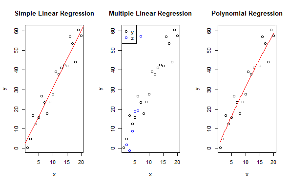
Proceed from Simple to Multiple and Polynomial Regression in R

This code plots the results of three different types of regressions: Simple Linear Regression, Multiple Linear Regression, and Polynomial Regression. It arranges the plots in one row with three columns using par. Each plot displays the relationship between predictor variables (x and z) and the response variable (y), along with the corresponding regression lines or curves. The plots are labeled with titles and axis labels for clarity. Finally, par(mfrow = c(1, 1)) resets the plotting layout to its default setting.

Conclusion

To proceed from simple to multiple and polynomial regression in R, begin with simple linear regression to understand the relationship between one independent variable and the dependent variable. Transition to multiple linear regression by incorporating additional independent variables for a more comprehensive analysis. If the relationship appears non-linear, consider polynomial regression by transforming the independent variable(s) into polynomial terms. Evaluate the goodness of fit and significance of each model using metrics like R-squared and p-values, then select the most appropriate model based on the complexity of the relationship and interpretability of results. This progressive approach enables a deeper understanding of variable relationships and enhances predictive accuracy.