Principal Components and Factor Analysis Using R

Factor analysis is a statistical technique used for dimensionality reduction and identifying the underlying structure (latent factors) in a dataset. It’s often applied in fields such as psychology, economics, and social sciences to understand the relationships between observed variables. Factor analysis assumes that observed variables can be explained by a smaller number of latent factors.

Factor Analysis

Here’s a step-by-step explanation of factor analysis, followed by an example in R:

Step 1: Data Collection

Collect data on multiple observed variables (also called indicators or manifest variables). These variables are usually measured on a scale and are hypothesized to be influenced by underlying latent factors.

Step 2: Assumptions of Factor Analysis

Factor analysis makes several assumptions, including:

• Linearity: The relationships between observed variables and latent factors are linear.
• No Perfect Multicollinearity: There are no perfect linear relationships among the observed variables.
• Common Variance: Observed variables share common variance due to latent factors.
• Unique Variance: Each observed variable also has unique variance unrelated to latent factors (measurement error).

Step 3: Factor Extraction

Factor extraction is the process of identifying the underlying latent factors. Common methods for factor extraction include Principal Component Analysis (PCA) and Maximum Likelihood Estimation (MLE). These methods extract factors that explain the most variance in the observed variables.

Step 4: Factor Rotation

After extraction, factors are often rotated to improve interpretability. Rotation methods (e.g., Varimax, Promax) help in achieving a simpler and more interpretable factor structure.

Step 5: Interpretation

Interpret the rotated factor loadings. Factor loadings represent the strength and direction of the relationship between each observed variable and each factor. High loadings indicate a strong relationship.

Step 6: Naming and Using Factors

Based on the interpretation of factor loadings, you can give meaningful names to the factors. These names help in understanding the underlying constructs. Researchers often use these factors in subsequent analyses.

Now, let’s see a code using R:

R

# Load necessary libraries
library(psych)

# Generate sample data with three latent factors
set.seed(123)
n <- 100
factor1 <- rnorm(n)
factor2 <- 0.7 * factor1 + rnorm(n)
factor3 <- 0.5 * factor1 + 0.5 * factor2 + rnorm(n)
observed1 <- 0.6 * factor1 + 0.2 * factor2 + rnorm(n)
observed2 <- 0.4 * factor1 + 0.8 * factor2 + rnorm(n)
observed3 <- 0.3 * factor1 + 0.5 * factor3 + rnorm(n)

# Create a data frame
data <- data.frame(observed1, observed2, observed3)

# Perform factor analysis
factor_analysis <- fa(data, nfactors = 3, rotate = "varimax")

# Print factor loadings
print(factor_analysis$loadings)

Output:

Loadings:
          MR1   MR2   MR3  
observed1 0.169 0.419      
observed2 0.574 0.544      
observed3 0.582 0.233      
                 MR1   MR2   MR3
SS loadings    0.697 0.526 0.000
Proportion Var 0.232 0.175 0.000
Cumulative Var 0.232 0.408 0.408

In this R example, we first generate sample data with three latent factors and three observed variables. We then use the `fa` function from the `psych` package to perform factor analysis. The output includes factor loadings, which indicate the strength and direction of the relationships between the observed variables and the latent factors.

Here’s a breakdown of the output:

• Standardized Loadings (Pattern Matrix): This section provides the factor loadings for each observed variable on the three extracted factors (MR1, MR2, and MR3). Factor loadings represent the strength and direction of the relationship between observed variables and latent factors.
• SS Loadings: These are the sum of squared loadings for each factor, indicating the proportion of variance in the observed variables explained by each factor.
• Proportion Var: This shows the proportion of total variance explained by each factor.
• Cumulative Var: This shows the cumulative proportion of total variance explained as more factors are added.

Factor Analysis on Iris Dataset

R

# Load the built-in iris dataset
data(iris)

# Perform factor analysis on the iris dataset
factanal_result <- factanal(iris[, 1:4], factors = 1, rotation = "varimax")

# Print the factor analysis results
print(factanal_result)

Output:

Call:
factanal(x = iris[, 1:4], factors = 1, rotation = "varimax")
Uniquenesses:
Sepal.Length  Sepal.Width Petal.Length  Petal.Width 
       0.240        0.822        0.005        0.069 
Loadings:
             Factor1
Sepal.Length  0.872 
Sepal.Width  -0.422 
Petal.Length  0.998 
Petal.Width   0.965 
               Factor1
SS loadings      2.864
Proportion Var   0.716
Test of the hypothesis that 1 factor is sufficient.
The chi square statistic is 85.51 on 2 degrees of freedom.
The p-value is 2.7e-19 

In this example, we use the built-in iris dataset, which contains measurements of sepal length, sepal width, petal length, and petal width for three species of iris flowers. We perform factor analysis on the first four columns of the dataset (the measurements) using the ‘factanal’ function.

The output includes:

• Uniquenesses: These values represent the unique variance in each observed variable that is not explained by the factors.
• Loadings: These values represent the factor loadings for each observed variable on the extracted factors. Positive and high loadings indicate a strong relationship.
• SS loadings, Proportion Var, and Cumulative Var: These statistics provide information about the variance explained by the extracted factors.
• Test of the hypothesis: This section provides a chi-square test of whether the selected number of factors is sufficient to explain the variance in the data.

Factor analysis helps in understanding the underlying structure of the iris dataset and can be useful for dimensionality reduction or creating composite variables for further analysis.

By interpreting these factor loadings, researchers can gain insights into the underlying structure of the data and potentially reduce the dimensionality for further analysis.

Unveiling Hidden Insights: Principal Components and Factor Analysis Using R

In the ever-evolving landscape of data analysis, the quest to uncover hidden patterns and reduce the dimensionality of complex datasets has led us to the intriguing realm of Principal Components and Factor Analysis. These techniques offer a lens through which we can distil the essence of our data, capturing its intrinsic structure and shedding light on the underlying relationships between variables. In this article, we embark on a journey to demystify Principal Components Analysis (PCA) and Factor Analysis (FA), exploring their concepts, steps, and implementation using the versatile R programming language.

Understanding the Foundation: Principal Components Analysis (PCA)

At its core, PCA is a dimensionality reduction technique that transforms high-dimensional data into a lower-dimensional space while preserving its variance. The first principal component captures the most significant variance, followed by subsequent components in decreasing order of variance. By representing data in a reduced space, PCA not only simplifies visualization but also aids in identifying dominant patterns and removing noise.

Factor Analysis: Peering into Latent Constructs

Factor Analysis, on the other hand, delves into understanding the underlying latent variables that contribute to observed variables. It seeks to unravel the common factors that influence the observed correlations and covariances in the dataset. These latent factors, which are not directly measurable, offer insights into the hidden structure governing the variables.

Steps to Illuminate Insights

1. Data Pre-processing: Start by preparing your data, ensuring that it is cleaned and standardized for accurate analysis.

R

# Load the iris dataset
data("iris")

# Standardize the data
standardized_data <- scale(iris[, 1:4])

2. Covariance or Correlation Matrix: Depending on the nature of your data, calculate either the covariance or correlation matrix. These matrices capture the relationships between variables.

R

# Calculate the correlation matrix
correlation_matrix <- cor(standardized_data)
print(correlation_matrix)

Output:

            Sepal.Length Sepal.Width Petal.Length Petal.Width
Sepal.Length    1.0000000  -0.1175698    0.8717538   0.8179411
Sepal.Width    -0.1175698   1.0000000   -0.4284401  -0.3661259
Petal.Length    0.8717538  -0.4284401    1.0000000   0.9628654
Petal.Width     0.8179411  -0.3661259    0.9628654   1.0000000

Correlation matrix of the standardized data can be found using the function “cor()”.

The output correlation_matrix will be a 4×4 matrix of correlation coefficients between variables.

3. Eigenvalue Decomposition: Employ eigenvalue decomposition to extract the principal components. R’s built-in functions like `eigen()` facilitate this process.

R

# Perform PCA using eigenvalue decomposition
pca_result <- eigen(correlation_matrix)
print(pca_result$values)

Output:

[1] 2.91849782 0.91403047 0.14675688 0.02071484

The eigen value decomposition of the correlation matrix can be done using the “eigen()” function.

R

# eigenvector decomposition
print(pca_result$vector)

Output:

           [,1]        [,2]       [,3]       [,4]
[1,]  0.5210659 -0.37741762  0.7195664  0.2612863
[2,] -0.2693474 -0.92329566 -0.2443818 -0.1235096
[3,]  0.5804131 -0.02449161 -0.1421264 -0.8014492
[4,]  0.5648565 -0.06694199 -0.6342727  0.5235971

The output will be a vector of eigenvalues.

4. Selecting Components: Determine the number of principal components to retain. This decision is based on the explained variance and the cumulative proportion it represents.

R

# Calculate the proportion of variance explained by each component
explained_variance <- pca_result$values / sum(pca_result$values)

# Cumulative proportion of variance explained
cumulative_proportion <- cumsum(explained_variance)

# Determine the number of components to retain
num_components <- sum(cumulative_proportion <= 0.95)
print(num_components)

Output:

1

• The code computes the proportion of variance explained by each principal component in the PCA result, dividing the eigenvalues by the sum of all eigenvalues.
• It calculates the cumulative proportion of variance explained by summing up the previously calculated explained variances.
• The code determines the number of principal components to retain by finding the count of cumulative proportions that are less than or equal to 0.95, ensuring that around 95% of the total variance is retained.

Number of components required, is the output in this case.

5. Interpreting Loadings: In the context of Factor Analysis, the factor loadings indicate the strength and direction of the relationship between the observed variables and the latent factors.

Install the psych package

install.packages("psych")

Code

R

# Load the psych package for factor analysis
library(psych)

# Perform factor analysis on the iris data
factor_result <- fa(standardized_data, nfactors = num_components, rotate = "varimax")

# Display factor loadings
print(factor_result$loadings)

Output:

Loadings:
             MR1   
Sepal.Length  0.823
Sepal.Width  -0.334
Petal.Length  1.015
Petal.Width   0.974
                 MR1
SS loadings    2.768
Proportion Var 0.692

• The code installs and loads the “psych” package, which is used for various psychological and statistical functions, including factor analysis.
• The code conducts factor analysis on the standardized data using the “fa” function. The “nfactors” parameter is set to the previously determined “num_components,” representing the number of principal components to retain. The “rotate” parameter specifies “varimax” rotation, a technique that simplifies factor loadings for better interpretation.
• The code prints the factor loadings obtained from the factor analysis. These loadings represent the relationships between observed variables and the latent factors extracted from the data. Each row corresponds to a variable, and each column corresponds to a factor, displaying the strength and direction of the relationship.
• This code segment essentially performs factor analysis on the standardized iris dataset and displays the factor loadings to uncover underlying latent factors that explain the variance in the data.

The output will be a matrix of factor loadings.

Let’s Walk Through with few Examples

Imagine a scenario where you’re analysing customer preferences across different product categories. You’ve gathered data on variables like purchase frequency, brand loyalty, and product reviews. Applying PCA or Factor Analysis can help you identify the key factors influencing customer behaviour.

Principal Components Analysis (PCA) using R with the built-in “USArrests” dataset

R

# Load the USArrests dataset
data("USArrests")

# Perform Principal Components Analysis
pca_result <- prcomp(USArrests, scale = TRUE)

pca_result

Output:

Standard deviations (1, .., p=4):
[1] 1.5748783 0.9948694 0.5971291 0.4164494
Rotation (n x k) = (4 x 4):
                PC1        PC2        PC3         PC4
Murder   -0.5358995 -0.4181809  0.3412327  0.64922780
Assault  -0.5831836 -0.1879856  0.2681484 -0.74340748
UrbanPop -0.2781909  0.8728062  0.3780158  0.13387773
Rape     -0.5434321  0.1673186 -0.8177779  0.08902432

Check the summary

R

# Print the summary of PCA
summary(pca_result)

Output:

Importance of components:
                          PC1    PC2     PC3     PC4
Standard deviation     1.5749 0.9949 0.59713 0.41645
Proportion of Variance 0.6201 0.2474 0.08914 0.04336
Cumulative Proportion  0.6201 0.8675 0.95664 1.00000

Now, we can print top 5 rows of the projected data

R

# Extract the loadings for the first two principal components
loadings <- pca_result$rotation[, 1:2]

# Project the original data onto the first two principal components
projected_data <- scale(USArrests) %*% loadings

# Display the first few rows of the projected data
print(head(projected_data))

Output:

                  PC1        PC2
Alabama    -0.9756604 -1.1220012
Alaska     -1.9305379 -1.0624269
Arizona    -1.7454429  0.7384595
Arkansas    0.1399989 -1.1085423
California -2.4986128  1.5274267
Colorado   -1.4993407  0.9776297

• Load Dataset: The code loads the built-in “USArrests” dataset, which contains crime statistics for different U.S. states.
• Perform PCA: It conducts Principal Components Analysis (PCA) on the “USArrests” data using the prcomp function. The parameter scale = TRUE standardizes the data before performing PCA.
• Print PCA Summary: The code prints a summary of the PCA result, displaying key information about the principal components, including their standard deviations and proportions of variance explained.
• Project Data: The original data is projected onto the first two principal components using the predict function applied to the PCA result.
• Display Projected Data: The code displays the first few rows of the projected data, which represents the original data transformed into the space of the first two principal components. This allows visualization and analysis in the reduced-dimensional space.

Identifying Dominant Features in Wine Data

R

# Load the wine dataset
wine_url <- "https://archive.ics.uci.edu/ml/machine-learning-databases/wine/wine.data"

wine <- read.table(wine_url, header = FALSE, sep = ",")

# Perform PCA
pca_result <- prcomp(wine, scale = TRUE)

# Proportion of variance explained by each component
print(summary(pca_result)$importance[3,])

Output:

    PC1     PC2     PC3     PC4     PC5     PC6     PC7     PC8     PC9    PC10 
0.39542 0.57379 0.67708 0.74336 0.80604 0.85409 0.89365 0.91865 0.93969 0.95843 
   PC11    PC12    PC13    PC14 
0.97456 0.98662 0.99587 1.00000 

• Load Dataset: The code loads the “wine” dataset, which contains measurements of chemical constituents in wines.
• Perform PCA: It conducts Principal Components Analysis (PCA) on the “wine” data using the prcomp function. The parameter scale = TRUE standardizes the data before performing PCA.
• Proportion of Variance Explained: The summary(pca_result)$importance[3,] code calculates the proportion of variance explained by each principal component. The summary function extracts information from the PCA result, and [3,] indexes the row that contains the proportions of variance explained.

Reducing Dimensionality of Iris Data

R

# Load the iris dataset
data("iris")

# Perform PCA
pca_result <- prcomp(iris[, 1:4], scale = TRUE)

# Variance explained by first two components
print(summary(pca_result)$importance[2,])

Output:

    PC1     PC2     PC3     PC4 
0.72962 0.22851 0.03669 0.00518 

• Load Dataset: The code loads the well-known “iris” dataset, which contains measurements of iris flowers.
• Perform PCA: It conducts Principal Components Analysis (PCA) on the first four columns of the “iris” dataset (features related to flower measurements) using the prcomp function. The parameter scale = TRUE standardizes the data before performing PCA.
• Variance Explained by First Two Components: The code calculates the variance explained by the first two principal components using summary(pca_result)$importance[2,]. The summary function extracts information from the PCA result, and [2,] indexes the row that contains the proportion of variance explained by the second principal component.

Analyzing Diabetes Diagnostics

R

diabetes <- read.csv('diabetes.csv')

# Perform PCA
pca_result <- prcomp(diabetes, scale = TRUE)

# Proportion of variance explained by each component
explained_variance <- pca_result$sdev^2
total_variance <- sum(explained_variance)
proportion_of_variance <- explained_variance / total_variance

# Display the proportion of variance explained by each component
print(proportion_of_variance)

Output:

[1] 0.26138907 0.19714578 0.12446946 0.09799499 0.09384705 0.08165203 0.05426927
[8] 0.04646457 0.04276780

• We load the built-in “diabetes” dataset, containing ten baseline variables related to diabetes diagnostics.
• Perform PCA on the dataset using the prcomp function with standardization.
• Calculate the proportion of variance explained by each component by squaring the standard deviations (sdev) of the components and dividing them by the total variance.
• The output displays the proportion of variance explained by each component.

Analyzing mtcars Dataset

R

# Load the mtcars dataset (built-in dataset in R)
data(mtcars)

# Perform PCA
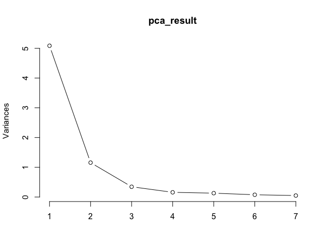
pca_result <- prcomp(mtcars[, 1:7], scale. = TRUE)

# Summary of PCA
summary(pca_result)

# Scree plot to visualize the variance explained by each principal component
plot(pca_result, type = "l")

library(psych)

# Perform Factor Analysis on selected columns of mtcars dataset
fa_result <- fa(mtcars[, c(1, 3, 4, 6, 7)], nfactors = 2)
print(fa_result)

# Extract eigenvalues from the Factor Analysis result
eigenvalues <- fa_result$values

print(eigenvalues)

Output:

Importance of components:
                          PC1    PC2     PC3     PC4    PC5     PC6     PC7
Standard deviation     2.2552 1.0754 0.58724 0.39741 0.3599 0.27542 0.22181
Proportion of Variance 0.7266 0.1652 0.04926 0.02256 0.0185 0.01084 0.00703
Cumulative Proportion  0.7266 0.8918 0.94107 0.96364 0.9821 0.99297 1.00000

Factor Analysis using method =  minres
Call: fa(r = mtcars[, c(1, 3, 4, 6, 7)], nfactors = 2)
Standardized loadings (pattern matrix) based upon correlation matrix
       MR1   MR2   h2      u2 com
mpg  -0.90 -0.13 0.84  0.1645 1.0
disp  0.93  0.13 0.87  0.1266 1.0
hp    0.90 -0.29 0.89  0.1128 1.2
wt    0.89  0.46 1.00 -0.0023 1.5
qsec -0.57  0.70 0.81  0.1931 1.9
                       MR1  MR2
SS loadings           3.58 0.82
Proportion Var        0.72 0.16
Cumulative Var        0.72 0.88
Proportion Explained  0.81 0.19
Cumulative Proportion 0.81 1.00
Mean item complexity =  1.3
Test of the hypothesis that 2 factors are sufficient.
df null model =  10  with the objective function =  5.51 with Chi Square =  156.89
df of  the model are 1  and the objective function was  0.02 
The root mean square of the residuals (RMSR) is  0 
The df corrected root mean square of the residuals is  0.01 
The harmonic n.obs is  32 with the empirical chi square  0.01  with prob <  0.93 
The total n.obs was  32  with Likelihood Chi Square =  0.47  with prob <  0.49 
Tucker Lewis Index of factoring reliability =  1.038
RMSEA index =  0  and the 90 % confidence intervals are  0 0.416
BIC =  -3
Fit based upon off diagonal values = 1
Measures of factor score adequacy             
                                                   MR1  MR2
Correlation of (regression) scores with factors   0.99 0.96
Multiple R square of scores with factors          0.98 0.93
Minimum correlation of possible factor scores     0.96 0.86
[1]  3.585855849  0.824286224  0.008494057 -0.001162944 -0.012187210

Now we print the Eigen Values

[1]  3.585855849  0.824286224  0.008494057 -0.001162944 -0.012187210

• We load the built-in “mtcars” dataset.
• Perform PCA on the dataset using the prcomp function with standardization.
• Plotting an Scree plot of the pca_result.
• Performing Factor Analysis on mtcars dataset.
• The output displays the Factor Analysis result along with the eigen values.

Output that Enlightens

Upon implementing PCA or Factor Analysis in R, you’ll be presented with insightful outcomes. For PCA, you’ll discover the proportion of variance captured by each component, aiding in dimensionality reduction decisions. In Factor Analysis, factor loadings unveil the relationship strengths, providing clues about latent variables shaping the observed data.

Conclusion

Principal Components and Factor Analysis empower us to sift through complex data, distilling essential insights that drive better decision-making. By implementing these techniques using R, we bridge the gap between raw data and meaningful patterns, uncovering the underlying structure that often remains hidden. As data scientists, we wield these tools to transform data into actionable knowledge, embracing the power of dimensionality reduction and latent factor discovery. So, embark on this journey, harness the capabilities of R, and unlock the secrets within your data.