Singular Value Decomposition (SVD)

The Singular Value Decomposition (SVD) of a matrix is a factorization of that matrix into three matrices. It has some interesting algebraic properties and conveys important geometrical and theoretical insights about linear transformations. It also has some important applications in data science. In this article, I will try to explain the mathematical intuition behind SVD and its geometrical meaning. 

Mathematics behind SVD:

The SVD of  mxn matrix A is given by the formula  

where:

• U:  mxm matrix of the orthonormal eigenvectors of .
• V^T: transpose of a nxn matrix containing the orthonormal eigenvectors of .
• : diagonal matrix with r elements equal to the root of the positive eigenvalues of AAᵀ or Aᵀ A (both matrics have the same positive eigenvalues anyway).

Examples

• Find the SVD for the matrix A = 
• To calculate the SVD, First, we need to compute the singular values by finding eigenvalues of AA^{T}.

• The characteristic equation for the above matrix is:

so our singular values are: 

• Now we find the right singular vectors i.e orthonormal set of eigenvectors of A^TA. The eigenvalues of A^TA are 25, 9, and 0, and since A^TA is symmetric we know that the eigenvectors will be orthogonal.

For 

which can be row-reduces to :

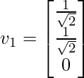
A unit vector in the direction of it is:

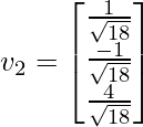
Similarly, for \lambda = 9, the eigenvector is:

For the 3rd eigenvector, we could use the property that it is perpendicular to v1 and v2 such that:

Solving the above equation to generate the third eigenvector

Now, we calculate U using the formula u_i = \frac{1}{\sigma} A v_i and this gives U =. Hence, our final SVD equation becomes:

Applications

• Calculation of Pseudo-inverse:  Pseudo inverse or Moore-Penrose inverse is the generalization of the matrix inverse that may not be invertible (such as low-rank matrices). If the matrix is invertible then its inverse will be equal to Pseudo inverse but pseudo inverse exists for the matrix that is not invertible. It is denoted by A⁺.

Suppose, we need to calculate the pseudo-inverse of a matrix M:
Then, the SVD of M can be given as:
Multiply both sides by M^{-1}.[Tex]I= M^{-1} U W V^{T}[/Tex]Multiply both side by V:[Tex]V = M^{-1} U W[/Tex]Multiply by W^{-1}Since the W is the singular matrix, the inverse of W  is [Tex]V W^{-1} =  M^{-1} U W W^{-1}[/Tex]Multiply by [Tex]V W^{-1} U^{T} = M^{-1} U U^{T}[/Tex]

The above equation gives the pseudo-inverse.

Solving a set of Homogeneous Linear Equation (Mx =b): if b=0,  calculate SVD and take any column of V^T associated with a singular value (in W) equal to 0.

If , Multiply by [Tex]M^{-1} M x = M^{-1} b [/Tex]

From the Pseudo-inverse, we know that 

Hence, 

• Rank, Range, and Null space: 
  • The rank of matrix M can be calculated from SVD by the number of nonzero singular values.
  • The range of matrix M is The left singular vectors of U corresponding to the non-zero singular values.
  • The null space of matrix M is The right singular vectors of V corresponding to the zeroed singular values.

• Curve Fitting Problem: Singular value decomposition can be used to minimize the least square error. It uses the pseudo inverse to approximate it.
• Besides the above application, singular value decomposition and pseudo-inverse can also be used in Digital signal processing and image processing

Implementation:

In this code, we will try to calculate the Singular value decomposition using Numpy and Scipy.  We will be calculating SVD, and also performing pseudo-inverse. In the end, we can apply SVD for compressing the image

Python3

# Imports

from skimage.color import rgb2gray
from skimage import data
import matplotlib.pyplot as plt
import numpy as np
from scipy.linalg import svd

"""
Singular Value Decomposition
"""
# define a matrix
X = np.array([[3, 3, 2], [2, 3, -2]])
print(X)
# perform SVD
U, singular, V_transpose = svd(X)
# print different components
print("U: ", U)
print("Singular array", singular)
print("V^{T}", V_transpose)

"""
Calculate Pseudo inverse
"""
# inverse of singular matrix is just the reciprocal of each element
singular_inv = 1.0 / singular
# create m x n matrix of zeroes and put singular values in it
s_inv = np.zeros(X.shape)
s_inv[0][0] = singular_inv[0]
s_inv[1][1] = singular_inv[1]
# calculate pseudoinverse
M = np.dot(np.dot(V_transpose.T, s_inv.T), U.T)
print(M)

"""
SVD on image compression
"""


cat = data.chelsea()
plt.imshow(cat)
# convert to grayscale
gray_cat = rgb2gray(cat)

# calculate the SVD and plot the image
U, S, V_T = svd(gray_cat, full_matrices=False)
S = np.diag(S)
fig, ax = plt.subplots(5, 2, figsize=(8, 20))

curr_fig = 0
for r in [5, 10, 70, 100, 200]:
    cat_approx = U[:, :r] @ S[0:r, :r] @ V_T[:r, :]
    ax[curr_fig][0].imshow(cat_approx, cmap='gray')
    ax[curr_fig][0].set_title("k = "+str(r))
    ax[curr_fig, 0].axis('off')
    ax[curr_fig][1].set_title("Original Image")
    ax[curr_fig][1].imshow(gray_cat, cmap='gray')
    ax[curr_fig, 1].axis('off')
    curr_fig += 1
plt.show()

Output:

[[ 3  3  2]
 [ 2  3 -2]]
---------------------------
U:  [[-0.7815437 -0.6238505]
 [-0.6238505  0.7815437]]
---------------------------
Singular array [5.54801894 2.86696457]
---------------------------
V^{T} [[-0.64749817 -0.7599438  -0.05684667]
 [-0.10759258  0.16501062 -0.9804057 ]
 [-0.75443354  0.62869461  0.18860838]]
--------------------------
# Inverse 
array([[ 0.11462451,  0.04347826],
       [ 0.07114625,  0.13043478],
       [ 0.22134387, -0.26086957]])
---------------------------

Original vs SVD k-image