Cost function in Logistic Regression in Machine Learning

Last Updated : 05 Dec, 2023

Logistic Regression is one of the simplest classification algorithms we learn while exploring machine learning algorithms. In this article, we will explore cross-entropy, a cost function used for logistic regression.

What is Logistic Regression?

Logistic Regression is a statistical method used for binary classification. Despite its name, it is employed for predicting the probability of an instance belonging to a particular class. It models the relationship between input features and the log odds of the event occurring, where the event is typically represented by the binary outcome (0 or 1).

The output of logistic regression is transformed using the logistic function (sigmoid), which maps any real-valued number to a value between 0 and 1. This transformed value can be interpreted as the probability of the instance belonging to the positive class.

Why do we need Logistic Regression?

Even when we have a linear regression algorithm, why do we need another logistic regression algorithm?

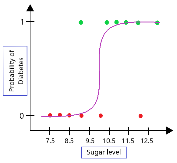
To answer this question first we need to understand the problem behind the linear regression for the classification task. Let’s consider an example of predicting diabetes based on sugar levels. In this example, we have a dataset with two variables: sugar levels (independent variable) and the likelihood of having diabetes (dependent variable, 1 for diabetic and 0 for non-diabetic).

linear-regression

As observed, the linear regression line ( $y=mx+c$ ) fails to accurately capture the relationship between sugar levels and the likelihood of diabetes. It assumes a linear relationship, which is not suitable for this binary classification problem. Extending this line will result in values that are less than 0 and greater than 1, which are not very useful in our classification problem.

This is where logistic regression comes into play, using the sigmoid function to model the probability of an instance belonging to a particular class.

Logistic function

Logistic function is also known as sigmoid function. It compressed the output of the linear regression between 0 & 1. It can be defined as:

$\sigma=\frac{1}{1+e^{-z^{(i)}}}$

Here, $z^{(i)} = h_\theta=\theta_1x_i+\theta_2$ is the linear combination of input features and model parameters.
The predicted probability $\sigma$ is the output of this sigmoid function.
e is the base of the natural logarithm, approximately equal to 2.718

When we applied the logistic functions to the output of the linear regression. it can be observed like:

As evident in the plot, sigmoid function is accurately separating the classes for binary classification tasks. Also, it produces continuous values exclusively within the 0 to 1 range, which can be employed for predictive purposes.

What is Cost Function?

A cost function is a mathematical function that calculates the difference between the target actual values (ground truth) and the values predicted by the model. A function that assesses a machine learning model’s performance also referred to as a loss function or objective function. Usually, the objective of a machine learning algorithm is to reduce the error or output of cost function.

When it comes to Linear Regression, the conventional Cost Function employed is the Mean Squared Error. The cost function (J) for m training samples can be written as:

$\begin{aligned} J(\theta) &= \frac{1}{2m} \sum_{i = 1}^{m} [z^{(i)} - y^{(i)}]^{2} \\ &= \frac{1}{2m} \sum_{i = 1}^{m} [h_{\theta}(x^{(i)}) - y^{(i)}]^{2} \end{aligned}$

where,

$y^{(i)}$ is the actual value of the target variable for the i-th training example.
$z^{(i)}=h_\theta(x^{(i)})$ is the predicted value of the target variable for the i-th training example, calculated using the linear regression model with parameters θ.
$x^{(i)}$ is the i-th training example.
m is number of training examples.

Plotting this specific error function against the linear regression model’s weight parameters results in a convex shape. This convexity is important because it allows the Gradient Descent Algorithm to be used to optimize the function. Using this algorithm, we can locate the global minima on the graph and modify the model’s weights to systematically lower the error. In essence, it’s a means of optimizing the model to raise its accuracy in making predictions.

Gradient-Descent-for-ML-Linear-Regression

Why Mean Squared Error cannot be used as cost function for Logistic Regression

Let’s consider the Mean Squared Error (MSE) as a cost function, but it is not suitable for logistic regression due to its nonlinearity introduced by the sigmoid function.

In logistic regression, if we substitute the sigmoid function into the above MSE equation, we get:

$\begin{aligned} J(\theta) &= \frac{1}{2m} \sum_{i = 1}^{m}[\sigma^{(i)} - y^{(i)}]^{2} \\&= \frac{1}{2m} \sum_{i=1}^{m} \left(\frac{1}{1 + e^{-z^{(i)}}} - y^{(i)}\right)^2 \\&= \frac{1}{2m} \sum_{i=1}^{m} \left(\frac{1}{1 + e^{-(\theta_1x^{(i)}+\theta_2)}} - y^{(i)}\right)^2 \end{aligned}$

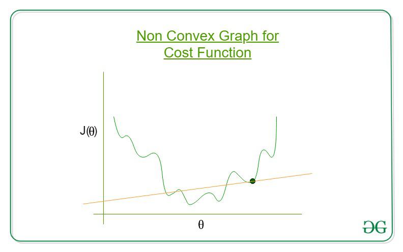
The equation $\frac{1}{1 + e^{-z}}$ is a nonlinear transformation, and evaluating this term within the Mean Squared Error formula results in a non-convex cost function. A non-convex function, have multiple local minima which can make it difficult to optimize using traditional gradient descent algorithms as shown below.

Cost_func_Non_Convex

Let’s break down the nonlinearity introduced by the sigmoid function and the impact on the cost function:

Sigmoid Function Nonlinearity

1. When z is large and positive, $e^z$ becomes very small, and $\frac{1}{1+e^{-z}}$ approaches 1.

Example:

when z=5,

$\begin{aligned} \frac{1}{1+e^{-5}}&= \frac{1}{{1+\frac{1}{e^{5}}}} \\ &=\frac{1}{(\frac{e^{5}+1}{e^{5}})} \\ &=\frac{e^{5}}{e^{5}+1} \\& = 0.9933071490757153 \end{aligned}$

Which is close to 1 indicating that the sigmoid function, when applied to a large positive value like 5, outputs a probability close to 1, suggesting a high confidence in the positive class.

2. When z is large and negative, $e^z$ dominates, and $\frac{1}{1+e^{-z}}$ approaches 0.

Example,

when z= -5, the expression becomes,

$\begin{aligned} \frac{1}{1+e^{-(-5)}}&= \frac{1}{1+e^{5}} \\& = 0.0066928509242848554 \end{aligned}$

Which is close to 0 indicating that sigmoid function, when applied to a large negative value like -5, outputs a probability close to 0. In other words, when z is a large negative number, the exponential term $e^z$ dominates the denominator, causing the sigmoid function to approach 0.

Squaring within the MSE Formula

The Mean Squared Error (MSE) formula involves squaring the difference between the predicted probability and the true label. In general Squaring the term $\frac{1}{1+e^{-z}}-y$ magnifies the errors when the predicted probability is far from the true label. but if the difference between the actual and predicted is in between 0 & 1 squaring the values will get lesser values.

Example 1:

If the true label y is 1 and the predicted probability $\frac{1}{{1+{e^{-z}}}} = 0.2$ ,

Squaring the difference :
$(1-0.2)^2= 0.8^2 = 0.64 <0.8$
Gives a lesser error than the predicted probability was, say, 0.8.

The squaring operation intensifies the impact of misclassifications, especially when $\hat{y}$  is close to 0 or 1.

While dealing with an optimization problem with Non-convex graph we face the problem of getting stuck at the local minima instead of the global minima. The presence of multiple local minima can make it challenging to find the optimal solution for a machine learning model. If the model gets trapped in a local minimum, it will not achieve the best possible performance. That’s where comes Log Loss or Cross Entropy Function most important term in the case of logistic regression.

Log Loss for Logistic regression

Log loss is a classification evaluation metric that is used to compare different models which we build during the process of model development. It is considered one of the efficient metrics for evaluation purposes while dealing with the soft probabilities predicted by the model.

The log of corrected probabilities, in logistic regression, is obtained by taking the natural logarithm (base e) of the predicted probabilities.

$\begin{aligned} \text{log loss} &= \ln{\sigma} \\ &= \ln{\frac{1}{1+e^{-z}}} \end{aligned}$

Let’s find the log odds for the examples, z=5

$\begin{aligned} \ln{(z=5)}&=\ln{\frac{1}{1+e^{-5}}} \\ &= \ln{\left (\frac{1}{{1+\frac{1}{e^{5}}}} \right )} \\ &=\ln{\left (\frac{e^{5}}{1+e^{5}} \right )} \\ &=\ln{e^5}-\ln{(1+e^5)} \\ &= 5 - \ln{(1+2.78^5)} \\ &= 5 - \ln{(1+2.71828^5)} \\ &= 5-5.006712007735388 \\&\approx -0.00671200 \end{aligned}$

and for z=-5,

$\begin{aligned} \ln{(z=-5)}&=\ln{\frac{1}{1+e^{-(-5)}}} \\ &= \ln{\left (\frac{1}{1+e^{5}} \right )} \\ &=\ln{1}-\ln{(1+e^5)} \\ &= 0 - \ln{(1+2.78^5)} \\ &= - \ln{(1+2.71828^5)} \\&\approx -5.00671200 \end{aligned}$

These log values are negative. In order to maintain the common convention that lower loss scores are better, we take the negative average of these values to deal with the negative sign.

Hence, The Log Loss can be summarized with the following formula:

$J = -\sum_{i=1}^{m}y_i\log \left ( h_\theta\left ( x_i \right ) \right ) + \left ( 1-y_i \right )\log \left (1- h_\theta\left ( x_i \right ) \right )$

where,

m is the number of training examples
$y_i$ is the true class label for the i-th example (either 0 or 1).
$h_\theta(x_i)$ is the predicted probability for the i-th example, as calculated by the logistic regression model.
$\theta$ is the model parameters

The first term in the sum represents the cross-entropy for the positive class ( $y_i = 1$ ), and the second term represents the cross-entropy for the negative class ( $y_i = 0$ ). The goal of logistic regression is to minimize the cost function by adjusting the model parameters $\theta$

In summary:

Calculate predicted probabilities using the sigmoid function.
Apply the natural logarithm to the corrected probabilities.
Sum up and average the log values, then negate the result to get the Log Loss.

Cost function for Logistic Regression

$Cost(h_{\theta}(x),y) = \left\{\begin{matrix} -log(h_{\theta}(x)) & if&y=1 \\ -log(1-h_{\theta}(x))& if& y = 0 \end{matrix}\right.$

Case 1: If y = 1, that is the true label of the class is 1. Cost = 0 if the predicted value of the label is 1 as well. But as h_θ(x) deviates from 1 and approaches 0 cost function increases exponentially and tends to infinity which can be appreciated from the below graph as well.
Case 2: If y = 0, that is the true label of the class is 0. Cost = 0 if the predicted value of the label is 0 as well. But as h_θ(x) deviates from 0 and approaches 1 cost function increases exponentially and tends to infinity which can be appreciated from the below graph as well.

download-(4)

With the modification of the cost function, we have achieved a loss function that penalizes the model weights more and more as the predicted value of the label deviates more and more from the actual label.

Conclusion

The choice of cost function, log loss or cross-entropy, is significant for logistic regression. It quantifies the disparity between predicted probabilities and actual outcomes, providing a measure of how well the model aligns with the ground truth.

Frequently Asked Questions (FAQs)

1. What is the difference between the cost function and the loss function for logistic regression?

The terms are often used interchangeably, but the cost function typically refers to the average loss over the entire dataset, while the loss function calculates the error for a single data point.

2.Why logistic regression cost function is non convex?

The sigmoid function introduces non-linearity, resulting in a non-convex cost function. It has multiple local minima, making optimization challenging, as traditional gradient descent may converge to suboptimal solutions.

3.What is a cost function in simple terms?

A cost function measures the disparity between predicted values and actual values in a machine learning model. It quantifies how well the model aligns with the ground truth, guiding optimization.

4.Is the cost function for logistic regression always negative?

No, the cost function for logistic regression is not always negative. It includes terms like -log(h(x)) and -log(1 – h(x)), and the overall value depends on the predicted probabilities and actual labels, yielding positive or negative values.

5.Why only sigmoid function is used in logistic regression?

The sigmoid function maps real-valued predictions to probabilities between 0 and 1, facilitating the interpretation of results as probabilities. Its range and smoothness make it suitable for binary classification, ensuring stable optimization.

Suggest improvement

Logistic Regression in Machine Learning

Share your thoughts in the comments