ML | Why Logistic Regression in Classification ?

Difficulty Level : Easy
Last Updated : 06 May, 2019

Using Linear Regression, all predictions >= 0.5 can be considered as 1 and rest all < 0.5 can be considered as 0. But then the question arises why classification can’t be performed using it?

Problem –

Suppose we are classifying a mail as spam or not spam and our output is y, it can be 0(spam) or 1(not spam). In case of Linear Regression, h_θ(x) can be > 1 or < 0. Although our prediction should be in between 0 and 1, the model will predict value out of the range i.e. maybe > 1 or < 0.

So, that’s why for a Classification task, Logistic/Sigmoid Regression plays its role.

$h_{\Theta} (x) = g (\Theta ^{T}x) z = \Theta ^{T}x g(z) = \frac{1}{1+e^{-z}}$

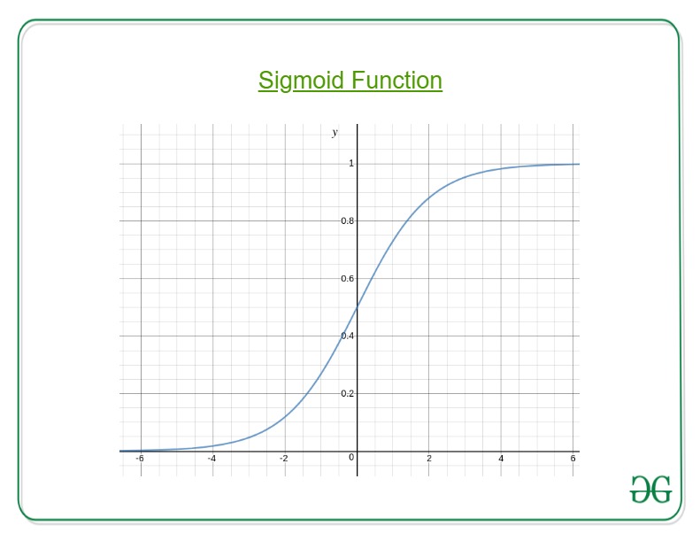
Here, we plug θ^Tx into logistic function where θ are the weights/parameters and x is the input and h_θ(x) is the hypothesis function. g() is the sigmoid function.

$h_{\Theta} (x) = P( y =1 | x ; \Theta )$

It means that y = 1 probability when x is parameterized to θ

To get the discrete values 0 or 1 for classification, discrete boundaries are defined. The hypothesis function cab be translated as

$h_{\Theta} (x) \geq 0.5 \rightarrow y = 1 h_{\Theta} (x) < 0.5 \rightarrow y = 0$

${g(z) \geq 0.5} \\ {\Rightarrow \Theta ^{T}x \geq 0.5} \\ {\Rightarrow z \geq 0.5 }$

Decision Boundary is the line that distinguishes the area where y=0 and where y=1. These decision boundaries result from the hypothesis function under consideration.

Understanding Decision Boundary with an example –
Let our hypothesis function be

$h_{\Theta}(x)= g[\Theta_{0}+ \Theta_1x_1+\Theta_2x_2+ \Theta_3x_1^2 + \Theta_4x_2^2 ]$

Then the decision boundary looks like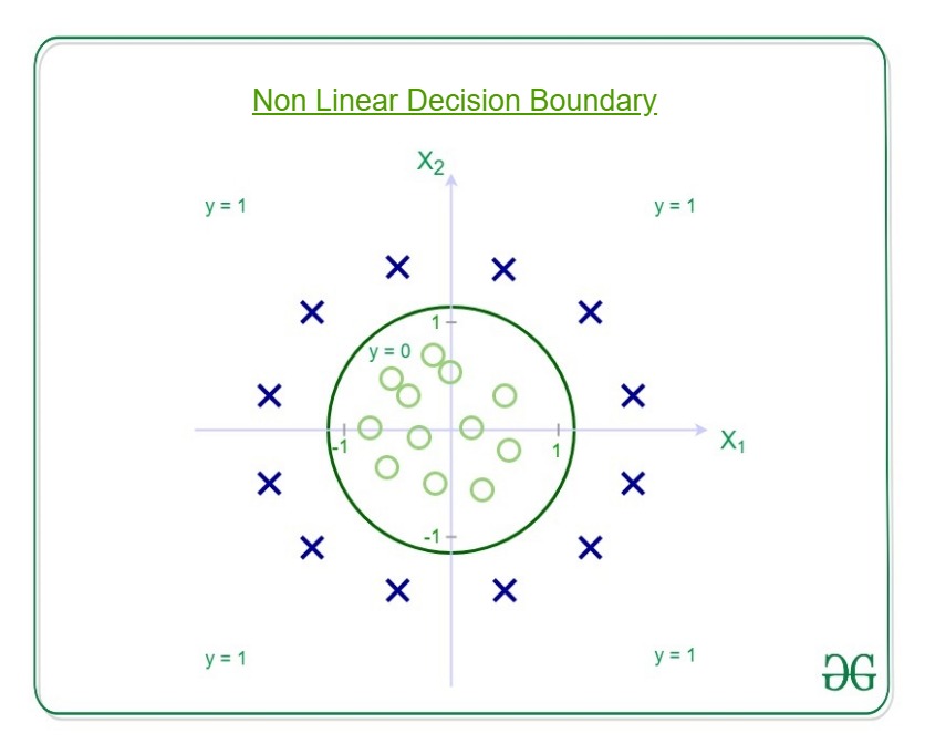

Let out weights or parameters be –

$\Theta=\begin{bmatrix} -1\\ 0\\ 0\\ 1\\ 1 \end{bmatrix}$

So, it predicts y = 1 if

$-1 + x_{1}^2 + x_{2}^2 \geqslant 0$

$\Rightarrow x_{1}^2 + x_{2}^2 \geqslant 1$

And that is the equation of a circle with radius = 1 and origin as the center. This is the Decision Boundary for our defined hypothesis.

Attention geek! Strengthen your foundations with the Python Programming Foundation Course and learn the basics.

To begin with, your interview preparations Enhance your Data Structures concepts with the Python DS Course. And to begin with your Machine Learning Journey, join the Machine Learning – Basic Level Course

My Personal Notes

Related Articles

ML | Why Logistic Regression in Classification ?