Linear Discriminant Analysis in R Programming
Last Updated :
10 Jul, 2020
One of the most popular or well established Machine Learning technique is Linear Discriminant Analysis (LDA ). It is mainly used to solve classification problems rather than supervised classification problems. It is basically a dimensionality reduction technique. Using the Linear combinations of predictors, LDA tries to predict the class of the given observations. Let us assume that the predictor variables are p. Let all the classes have an identical variant (i.e. for univariate analysis the value of p is 1) or identical covariance matrices (i.e. for multivariate analysis the value of p is greater than 1).
Method of implementing LDA in R
LDA or Linear Discriminant Analysis can be computed in R using the lda() function of the package MASS. LDA is used to determine group means and also for each individual, it tries to compute the probability that the individual belongs to a different group. Hence, that particular individual acquires the highest probability score in that group.
To use lda() function, one must install the following packages:
- MASS package for
lda() function.
- tidyverse package for better and easy data manipulation and visualization.
- caret package for a better machine learning workflow.
On installing these packages then prepare the data. To prepare data, at first one needs to split the data into train set and test set. Then one needs to normalize the data. On doing so, automatically the categorical variables are removed. Once the data is set and prepared, one can start with Linear Discriminant Analysis using the lda() function.
At first, the LDA algorithm tries to find the directions that can maximize the separation among the classes. Then it uses these directions for predicting the class of each and every individual. These directions are known as linear discriminants and are a linear combinations of the predictor variables.
Explanation of the function lda()
Before implementing the linear discriminant analysis, let us discuss the things to consider:
- One needs to inspect the univariate distributions of each and every variable. It must be normally distributed. If not, then transform using either the log and root function for exponential distribution or the Box-Cox method for skewed distribution.
- One needs to remove the outliers of the data and then standardize the variables in order to make the scale comparable.
- Let us assume that the dependent variable i.e. Y is discrete.
- LDA assumes that the predictors are normally distributed i.e. they come from gaussian distribution. Various classes have class specific means and equal covariance or variance.
Under the MASS package, we have the lda() function for computing the linear discriminant analysis. Let’s see the default method of using the lda() function.
Syntax:
lda(formula, data, …, subset, na.action)
Or,
lda(x, grouping, prior = proportions, tol = 1.0e-4, method, CV = FALSE, nu, …)
Parameters:
formula: a formula which is of the form group ~ x1+x2..
data: data frame from which we want to take the variables or individuals of the formula preferably
subset: an index used to specify the cases that are to be used for training the samples.
na.action: a function to specify that the action that are to be taken if NA is found.
x: a matrix or a data frame required if no formula is passed in the arguments.
grouping: a factor that is used to specify the classes of the observations.prior: the prior probabilities of the class membership.
tol: a tolerance that is used to decide whether the matrix is singular or not.
method: what kind of methods to be used in various cases.
CV: if it is true then it will return the results for leave-one-out cross validation.
nu: the degrees of freedom for the method when it is method=”t”.
…: the various arguments passed from or to other methods.
The function lda() has the following elements in it’s output:
- Prior possibilities of groups i.e. in each and every group the proportion of the training observations.
- Group means i.e. the group’s center of gravity and is used to show in a group the mean of each and every variable.
- Coefficients of linear discriminants i.e the linear combination of the predictor variables which are used to form the decision rule of LDA.
Example:
Let us see how Linear Discriminant Analysis is computed using the lda() function. Let’s use the iris data set of R Studio.
library(MASS)
library(tidyverse)
library(caret)
theme_set(theme_classic())
data("iris")
set.seed(123)
training.individuals <- iris$Species %>%
createDataPartition(p = 0.8, list = FALSE)
train.data <- iris[training.individuals, ]
test.data <- iris[-training.individuals, ]
preproc.parameter <- train.data %>%
preProcess(method = c("center", "scale"))
train.transform <- preproc.parameter %>% predict(train.data)
test.transform <- preproc.parameter %>% predict(test.data)
model <- lda(Species~., data = train.transform)
predictions <- model %>% predict(test.transform)
mean(predictions$class==test.transform$Species)
model <- lda(Species~., data = train.transform)
model
|
Output:
[1] 1
Call: lda(Species ~ ., data = train.transformed)

Prior probabilities of groups:
    setosa versicolor  virginica
 0.3333333  0.3333333  0.3333333

Group means:
           Sepal.Length Sepal.Width Petal.Length Petal.Width
setosa       -1.0120728   0.7867793   -1.2927218  -1.2496079
versicolor    0.1174121  -0.6478157    0.2724253   0.1541511
virginica     0.8946607  -0.1389636    1.0202965   1.0954568

Coefficients of linear discriminants:
                    LD1         LD2
Sepal.Length  0.9108023  0.03183011
Sepal.Width   0.6477657  0.89852536
Petal.Length -4.0816032 -2.22724052
Petal.Width  -2.3128276  2.65441936

Proportion of trace:
   LD1    LD2
0.9905 0.0095
Graphical plotting of the output
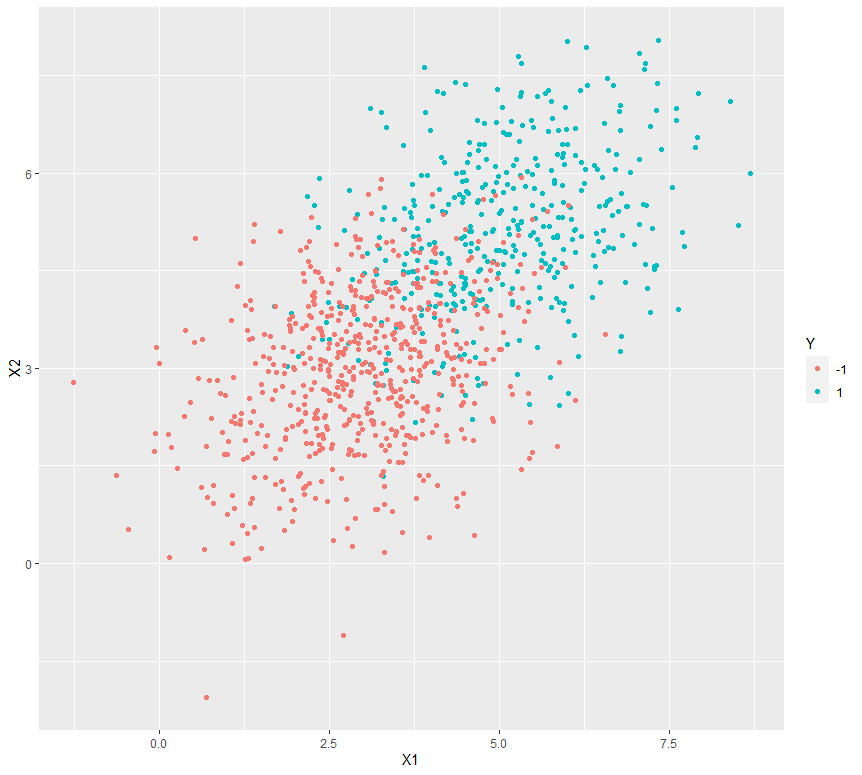
Let’s see what kind of plotting is done on two dummy data sets. For this let’s use the ggplot() function in the ggplot2 package to plot the results or output obtained from the lda().
Example:
library(ggplot2)
library(MASS)
library(mvtnorm)
var_covar = matrix(data = c(1.5, 0.4, 0.4, 1.5), nrow = 2)
Xplus1 <- rmvnorm(400, mean = c(5, 5), sigma = var_covar)
Xminus1 <- rmvnorm(600, mean = c(3, 3), sigma = var_covar)
Y_samples <- c(rep(1, 400), rep(-1, 600))
dataset <- as.data.frame(cbind(rbind(Xplus1, Xminus1), Y_samples))
colnames(dataset) <- c("X1", "X2", "Y")
dataset$Y <- as.character(dataset$Y)
ggplot(data = dataset) + geom_point(aes(X1, X2, color = Y))
|
Output:
Applications
- In Face Recognition System, LDA is used to generate a more reduced and manageable number of features before classifications.
- In Customer Identification System, LDA helps to identify and choose the features which can be used to describe the characteristics or features of a group of customers who can buy a particular item or product from a shopping mall.
- In field of Medical Science, LDA helps to identify the features of various diseases and classify it as mild or moderate or severe based on the patient’s symptoms.
Share your thoughts in the comments
Please Login to comment...