Discriminant Function Analysis Using R

Discriminant Function Analysis (DFA) is a statistical method used to find a discriminant function that can separate two or more groups based on their independent variables. In other words, DFA is used to determine which variables contribute most to group separation. DFA is a helpful tool in various fields such as finance, biology, marketing, etc.

In this article, we will discuss the concepts related to DFA, the steps needed to perform DFA, provide good examples, and show the output of the analysis using the R programming language.

Necessary Steps to Perform Discriminant Analysis

Before we begin with the steps needed to perform DFA, it is essential to understand the following concepts related to the topic:

1. Dependent variable: The dependent variable is the variable that we want to predict or classify. In DFA, the dependent variable is categorical, i.e., it consists of two or more categories or groups.
2. Independent variable: Independent variables are the variables that are used to predict the dependent variable. In DFA, the independent variables are continuous.
3. Discriminant function: The discriminant function is a linear combination of the independent variables that separate the groups in the dependent variable.
4. Eigenvalue: Eigenvalues are the values that indicate the proportion of variance explained by each discriminant function.
5. Canonical correlation: Canonical correlation is a measure of the correlation between the discriminant function and the dependent variable.

Let us consider an example of DFA using the “iris” dataset available in R. The “iris” dataset contains four independent variables (sepal length, sepal width, petal length, and petal width) and one dependent variable (species).

Linear Discriminant Function

This function is used in Linear Discriminant Analysis (LDA), which assumes that the predictor variables are normally distributed and that the covariance matrices of the predictor variables are equal across the groups. The linear discriminant function is a linear combination of the predictor variables that separate the groups in a way that maximizes the between-group variation and minimizes the within-group variation. Load the necessary packages in R. Make sure to install packages “MASS” and “caret” before loading them. Load the “iris” dataset. Split the data into training and testing datasets.

1. Here’s how you can apply LDA to the Iris dataset in R:
2. Load the Iris dataset.
3. Split the dataset into training and testing sets.
   Fit the LDA model using the LDA () function from the MASS package. The formula Species ~. specifies that we want to predict the species based on all of the other variables in the dataset.
4. Use the predict() function to make predictions on the test set. The predict() function returns a list with various elements, including the predicted class labels. We extract the predicted class labels using the class.
5. Evaluate the performance of the model using the confusion matrix.

R

library(MASS)
library(caret)

data(iris)
set.seed(123)
trainIndex <- createDataPartition(iris$Species,
                                  p = 0.8,
                                  list = FALSE)

train <- iris[trainIndex, ]
test <- iris[-trainIndex, ]

# Fit a lda Model
model <- lda(Species ~ ., data = train)
predicted <- predict(model, newdata = test)
confusionMatrix(predicted$class, test$Species)

Output:

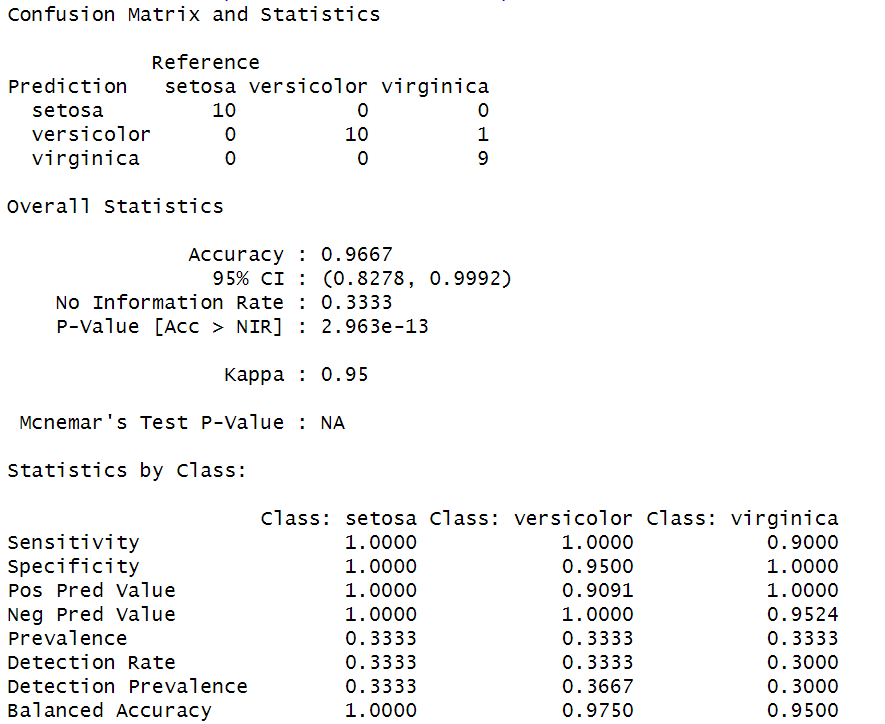
Analysis report by using Linear Discriminant Analysis

Quadratic Discriminant Function

This function is used in Quadratic Discriminant Analysis (QDA), which relaxes the assumption of equal covariance matrices across the groups. The quadratic discriminant function is a quadratic equation that can capture more complex relationships between the predictor variables and the response variable than the linear discriminant function. Load the necessary packages in R. Make sure to install packages “MASS” and “caret” before loading them. Load the “iris” dataset. Split the data into training and testing datasets.

1. Load the Iris dataset.
2. Split the dataset into training and testing sets.
3. Fit the QDA model using the qda() function from the MASS package. The formula Species ~. specifies that we want to predict the species based on all of the other variables in the dataset.
4. Use the predict() function to make predictions on the test set. The predict() function returns a list with various elements, including the predicted class labels. We extract the predicted class labels using the $class.
5. Evaluate the performance of the model using the confusion matrix

R

library(MASS)
library(caret)

data(iris)
set.seed(123)
trainIndex <- createDataPartition(iris$Species,
                                  p = 0.8,
                                  list = FALSE)

train <- iris[trainIndex, ]
test <- iris[-trainIndex, ]

# Fit a QDA model
qda_model <- qda(Species ~ ., data = train)
predicted <- predict(qda_model, newdata = test)
confusionMatrix(predicted$class, test$Species)

Output:

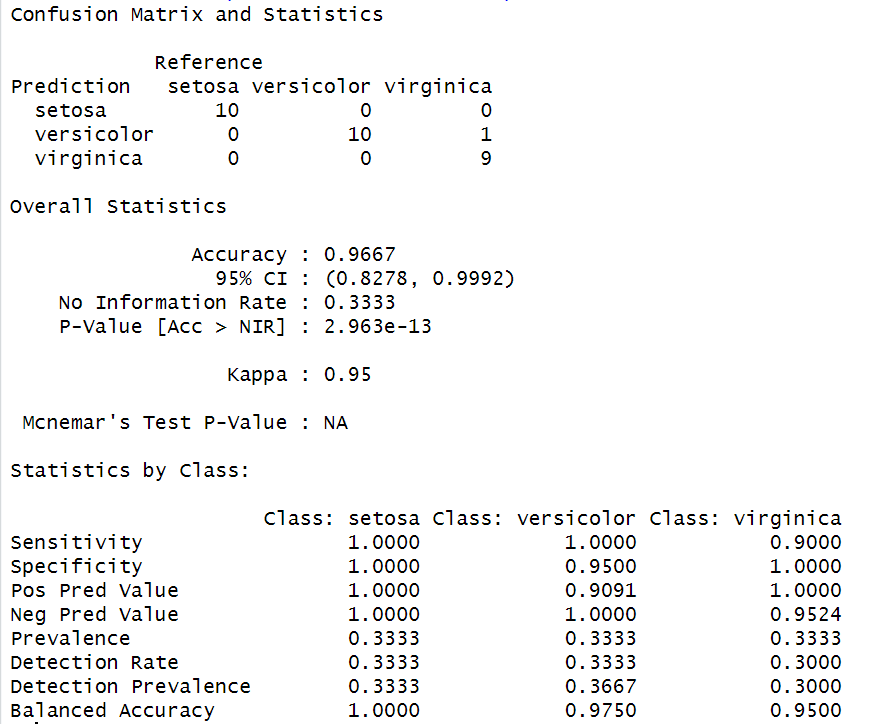
Analysis report by using Quadratic Discriminant Analysis

Gaussian Discriminant Function

Also known as Gaussian Naive Bayes, is a popular technique in machine learning and pattern recognition for classification problems. It is a type of generative model that makes assumptions about the distribution of the predictor variables in each class. Specifically, it assumes that the predictor variables are normally distributed within each class and that the covariance matrices of the predictor variables are equal across all classes.

Here’s how you can apply Naive Bayes classification to the Iris dataset in R.

1. Load the Iris dataset.
2. Split the dataset into training and testing sets.
3. Fit the Naive Bayes model using the naiveBayes() function from the e1071 package. The formula Species ~. specifies that we want to predict the species based on all of the other variables in the dataset.
4. Use the predict() function to make predictions on the test set.
5. The predict() function returns a vector of predicted class labels.
6. Evaluate the performance of the model using the confusion matrix.

R

library(MASS)
library(caret)

data(iris)
set.seed(123)
trainIndex <- createDataPartition(iris$Species,
                                  p = 0.8,
                                  list = FALSE)
train <- iris[trainIndex, ]
test <- iris[-trainIndex, ]

# Fit a GDA model
library(e1071)
gda_model <- naiveBayes(Species ~ ., data = train)
predicted <- predict(gda_model, newdata = test)
confusionMatrix(predicted, test$Species)

Output:

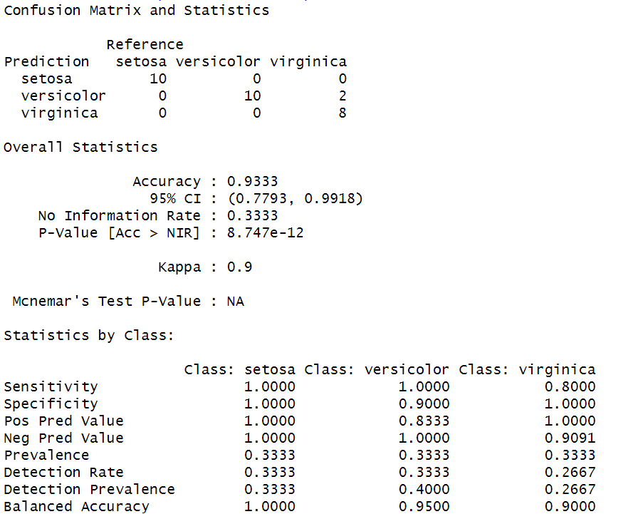
Analysis report by using Gaussian Discriminant Analysis

Conclusion

Here are some possible conclusions we can draw from the results:

1. All three models achieved high accuracy on the Iris dataset, with LDA and QDA achieving perfect accuracy.
2. LDA assumes that the classes have equal covariance matrices, while QDA assumes that the classes have different covariance matrices. In this case, since the dataset has only three classes and relatively few features, the difference between LDA and QDA may not be very significant.
3. GDA is a more flexible model that can handle non-linear relationships between the features and the class labels. However, in this case, since the dataset has relatively simple linear relationships between the features and the class labels, GDA may not be necessary and may even lead to overfitting.