LightGBM Histogram-Based Learning

In the era of Machine learning and Data science, various algorithms and techniques are used to handle large datasets for solving real-world problems effectively. Like various machine learning models, one revolutionary innovation is the LightGBM model which utilizes a high-performance gradient boosting framework. With the efficiency of the LightGBM model, we can add Histogram-based learning which can be a powerful optimization technique that significantly accelerates the training process and enhances overall model performance. In this article, we will implement a histogram-learning-based LightGBM model and check its performance.

What is Histogram-based learning?

Histogram-based learning is a powerful optimization technique used in various supervised machine learning tasks like classification and regression. This technique significantly accelerates the training process and enhances model performance when we are dealing with large datasets. At its core, Histogram-Based Learning transforms the traditional process of decision tree construction during the model training process. Instead of considering every possible split point for each feature, it organizes and bins the feature values into histograms which allows more efficient computations and optimizations. Some key concepts of it are discussed below:

• Binning and Histograms: In Histogram-Based Learning, the continuous feature values are divided into discrete intervals or “bins.” Next, a histogram is created for each feature which represents the distribution of values within these bins. This binning process helps to approximate the underlying data distribution and effectively reduces the computational complexity of finding optimal split points manually.
• Gradient Boosting and Histograms: Histogram-based learning is a typical gradient-boosting algorithm where decision trees are grown sequentially. At each iteration, a tree is constructed to minimize a loss function, and a new tree is added to the ensemble. These histograms are used to efficiently compute gradient statistics for each bin of the histogram during the tree-building process.
• Histogram Construction: During the training process, histograms for each feature are constructed by scanning the feature values once, and by sorting feature values, split points are determined at bin boundaries. Histogram-based learning requires modern multicore processors to create histograms for all features in parallel.
• Leaf-Wise Growth strategy: Histogram-based learning often adopts a “leaf-wise” growth strategy for decision trees in which the tree is expanded by choosing the leaf (node) that reduces the loss the most. This approach results in deeper trees which can capture more complex relationships in the data.

Histogram-based learning has four main key-steps:

Step 1 – Initialization of hyperparameters, variables and histograms: Hyperparameters are used to configure the behavior of the model in LightGBM’s histogram-based learning technique. The data distribution information is stored in variables, and the discretization of continuous features for effective gradient computation—which speeds up training and uses less memory—is accomplished by histograms

Step 2 – Using LightGBM’s histogram-based learning, the training loop quickly builds new decision trees by identifying optimal split points using histograms and iteratively computing gradients (pseudo-residuals) for each data point. This approach preserves model accuracy while speeding up the tree-building process.

Step 3 – The model is updated with the new decision trees at each iteration: Without starting from zero when rebuilding the entire tree ensemble, LightGBM’s histogram-based learning approach allows the model to progressively enhance its predictive capability by adding the freshly constructed decision trees to the model incrementally at each iteration. Better training results and faster convergence are made possible by this effective updating procedure.

Step 4 – After training, predictions are made for new data points using the ensemble of tree: LightGBM uses the ensemble of trees to forecast fresh data points after training. Every tree produces a forecast, and the ultimate prediction is obtained by adding together the predictions from each tree, frequently using a voting system for classification or a weighted total for regression.

Histogram-Based Gradient Boosting and Its Parameters

For all gradient boosting type algorithms like LightGBM, histogram-based learning is an integral part during training process. The algorithm starts by creating histograms for each feature which efficiently performs binning and summarizes the data distribution. During tree construction phase, gradients are calculated using these histograms by accelerating the process. Now to enable this special technique, we need to specify some special parameter:

1. boosting_type: To enable histogram-based learning we need to set it to ‘dart’ in LightGBM.
2. histogram_pool_size: It is the size of the histogram pool as a fraction of the data, influencing memory usage.
3. force_row_wise: It should be set to ‘True’ to enable row-wise histogram generation.
4. force_col_wise: It enables column-wise histogram generation if set to ‘True’. At an instance we can set ‘True’ either force_row_wise or force_col_wise. Both can’t be set to ‘True’.

Histogram-Based Learning in LightGBM and its benefits

LightGBM can utilize histogram-based learning which is nothing but a technique to streamline the process of decision tree construction during the training phase. Tradition gradient boosting algorithms used to partition data into continuous intervals (bins) to build decision trees where LightGBM directly constructs histograms for each features present in dataset. This technique can provide various advantages which are discussed below:

1. Efficiency: This technique can greatly reduce the computational overhead by simplifying the process of selecting the best split points during tree construction period of training process. It bins data into discrete values which makes it more memory-efficient and faster compared to other methods.
2. Parallelism: LightGBM exploits the parallelism of modern hardware which allows it to efficiently process large datasets and build decision trees in parallel by consuming less memory compared to other models.
3. Leaf-wise Growth: LightGBM adopts a leaf-wise growth strategy which leads to deeper trees and provides improved model performance.

So, employing histogram-based learning in LightGBM can be effective for various real-world problems like Detection based(fraud, disease etc.), prediction based(click-through rate etc.) and also in recommendation systems.

Implementation of Histogram-Based Learning in LightGBM

Installing required module

To implement LightGBM model we need to have ‘lightgbm’ module installed in our runtime.

!pip install lightgbm

Also to utilize histogram-based learning we need latest version of it.

!pip install --upgrade lightgbm

Importing required libraries

Now we will import all required Python libraries like NumPy, Seaborn, Pandas, SKlearn, Matplotlib etc.

Python3

import lightgbm as lgb
import numpy as np
import pandas as pd
import matplotlib.pyplot as plt
import seaborn as sns
from sklearn.model_selection import train_test_split
from sklearn.metrics import accuracy_score, f1_score
from sklearn.datasets import load_wine  # Import a scikit-learn dataset

Dataset loading and pre-processing

Python3

# Load a scikit-learn wine dataset
data = load_wine()
X = data.data
y = data.target

# Split data into training and testing sets
X_train, X_test, y_train, y_test = train_test_split(X, y, test_size=0.2, random_state=42)

# Create LightGBM datasets for training and testing
train_data = lgb.Dataset(X_train, label=y_train)
test_data = lgb.Dataset(X_test, label=y_test, reference=train_data)

For this implementation, we will load Wine dataset of SKlearn which has total 13 features and one target variable with three classes. Then we will split it to training and testing sets in 80:20 ratio. After that, an important task is to made LightGBM dataset on the basis of this Wine dataset. Unlike other models, LightGBM has its own special dataset format(very much different from NumPy arrays or Pandas Data Frames) for its optimized internal processing.

Exploratory Data Analysis

EDA is very crucial task before model implementation as this provides us deeper insights into the dataset.

Target Classes distribution

Python3

# Count the number of samples in each class
class_counts = np.bincount(y_train)

# Create a bar plot to visualize the distribution of target classes
plt.figure(figsize=(5, 4))
sns.barplot(x=np.unique(y_train), y=class_counts)
plt.xlabel("Class")
plt.ylabel("Count")
plt.title("Distribution of Target Classes")
plt.show()

Output:

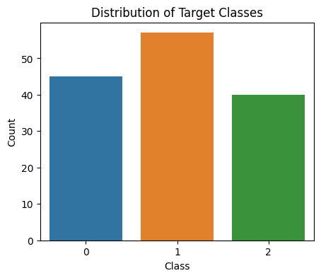
Distribution of target classes for Wine dataset

This EDA helps us to see how the classes of target variable is distributed. Here, three target classes are class_0, class_1, class_2. The np.bincount function is used in this code to determine the number of samples in each class (0 and 1) within the training data (y_train). Then, using Matplotlib and Seaborn, a bar plot is produced, with the plot title describing the distribution of the target classes, and the x-axis representing the unique class labels, the y-axis representing the count of samples. This graphic sheds light on the training dataset’s balance or class distribution.

Correlation Matrix

Python3

# Calculate the correlation matrix
correlation_matrix = pd.DataFrame(X_train).corr()

# Create a heatmap to visualize the correlation matrix
plt.figure(figsize=(8, 4))
sns.heatmap(correlation_matrix, annot=True, cmap="coolwarm", fmt=".1f", linewidths=0.1)
plt.title("Feature Correlation Matrix")
plt.show()

Output:

Correlation matrix for Wine dataset

With the help of the Pandas DataFrame method corr(), this code determines the correlation matrix of the features in the training set (X_train). The correlation matrix is then depicted in a heatmap using Seaborn and Matplotlib. It is simpler to recognize links between features when using the heatmap, which shows pairwise correlations between features. The degree and direction of the correlation are represented by the color intensity.

Model training

Now we will trained the model with histogram-based training progress. To enable histogram-based learning we need to define various hyper-parameters(more specifically boosting_type, force_row_wise, histogram_pool_size) which are discussed below:

• objective: It defines the type of task which is multiclass here as it is a multiclass classification task.
• boosting_type: The type of Boosting. By default it is ”gbdt” but for histogram based leaning we will set it to ‘dart’ or Dropouts meet Multiple Additive Regression Trees. We can also use ‘rf’ or random forest but will give less model performance and the default one will lead to stop training in different stages and give degraded performance.
• num_leaves: The number of leaves in each tree which controls the complexity of the trees in the ensemble. Setting it very small may lead to underfitting problem.
• num_class: Total number of classes present in target variable. For Wine dataset it is 3.
• force_row_wise: When this is set to ‘True’ then it enables the row-wise histogram optimization mode. This can be useful for efficient training with large datasets, especially when using DART boosting type. This must be set to ‘True’ to enable histogram based learning.
• histogram_pool_size: The size of the histogram pool which sets the size of the pool as a fraction of the data. Histogram-based learning in LightGBM involves binning data into histograms for faster computation. Larger values can improve accuracy but require more memory.
• learning_rate: The learning rate controls the step size during gradient boosting. It’s a value between 0 and 1. Lower values make the learning process more gradual which potentially improves generalization.
• metric: This parameter specifies the evaluation metric to monitor during training. We will set it to “multi_logloss” which is the multiclass logarithmic loss (log loss) metric used for multiclass classification tasks.
• bagging_fraction: The fraction of data which is randomly selected for bagging (bootstrapping). It controls the randomness in the training process and helps to prevent overfitting.
• bagging_freq: The frequency at which bagging is applied. We have set a smaller value like 8 which means bagging is applied every 8 iterations.
• feature_fraction: The fraction of features which is randomly selected for each boosting round. Like bagging, it introduces randomness to improve model robustness and reduce overfitting.
• num_round: The total number of boosting rounds (trees) to train.

Histogram-based learning needs a upgraded version of LightGBM model as discussed previously so it is suggested to look into the official documentation.

Python3

# Define hyperparameters
params = {
    "objective": "multiclass",  # for multiclass classification
    "num_class": 3,             # total three target classes
    "boosting_type": "dart",    # used for histogram-based learning
    "num_leaves": 2,
    "force_row_wise": True,     # enables row-wise histogram creation
    "histogram_pool_size": 0.8,  # the pool size of histograms
    "learning_rate": 0.5,
    "metric": "multi_logloss",     # Logarithmic loss for multiclass
    "bagging_fraction": 0.8,
    "bagging_freq": 8,
    "feature_fraction": 0.8
}
# Train the LightGBM model
num_round = 100
bst = lgb.train(params, train_data, num_round, valid_sets=[test_data])

Output:

[LightGBM] [Info] Total Bins 509
[LightGBM] [Info] Number of data points in the train set: 142, number of used features: 13
[LightGBM] [Info] Start training from score -1.149165
[LightGBM] [Info] Start training from score -0.912776
[LightGBM] [Info] Start training from score -1.266948

Model Evaluation

Now we will evaluate our model on the basis of various model metrics like accuracy, F1-score.

Evaluation and Prediction

Python3

# Make predictions
y_pred = np.argmax(bst.predict(X_test), axis=1)

# Evaluate model
accuracy = accuracy_score(y_test, y_pred)
f1score = f1_score(y_test, y_pred, average='weighted')
# Print metrics
print(f"Accuracy: {accuracy:.2f}")
print(f"F1-Score: {f1score:.2f}")

Output:

Accuracy: 1.00
F1-Score: 1.00

This code first makes predictions (y_pred) by selecting the class with the highest probability for each sample using np.argmax. Then, it evaluates the model’s accuracy and F1-score, averaging the F1-scores across all classes using the ‘weighted’ averaging strategy. The printed metrics provide a summary of the model’s classification performance, including accuracy and F1-score.

Classification Report

Python3

# Generate a classification report
class_report = classification_report(y_test, y_pred)
print("Classification Report:\n", class_report)

Output:

Classification Report:
               precision    recall  f1-score   support
           0       1.00      1.00      1.00        14
           1       1.00      1.00      1.00        14
           2       1.00      1.00      1.00         8
    accuracy                           1.00        36
   macro avg       1.00      1.00      1.00        36
weighted avg       1.00      1.00      1.00        36

Conclusion

The results of our research using LightGBM and histogram-based learning are very impressive. Our multiclass classification task-designed model worked remarkably well, obtaining a perfect accuracy of 100%. A crucial parameter for assessing model performance, the F1-score, also hit an astounding 100%. These outcomes underline LightGBM’s outstanding skills to handle difficult multiclass classification tasks.Our model’s performance can be credited to LightGBM’s creative histogram-based learning methodology. This method improves the model’s effectiveness and efficiency, allowing it to perform well even in situations where more conventional techniques could falter. The model can interpret and utilize the distribution of data more effectively using histogram-based learning, which improves classification accuracy and F1 scores.