Train a model using LightGBM

Light Gradient Boosting Machine (LightGBM) is an open-source and distributed gradient boosting framework that was developed by Microsoft Corporation. Unlike other traditional machine learning models, LightGBM can efficiently large datasets and has optimized training processes. LightGBM can be employed in classification, regression, and also in ranking tasks. For these reasons, LightGBM became very popular among Data Scientists and Machine learning researchers.

LightGBM

LightGBM is a gradient-boosting ensemble technique based on decision trees. LightGBM can be used for both classification and regression, just like other decision tree-based techniques. LightGBM is designed for great performance in distributed systems.LightGBM builds decision trees that develop leaf-wise, which implies that given a condition, just one leaf is split, depending on the benefit. Sometimes, especially with smaller datasets, leaf-wise trees might overfit. Overfitting can be prevented by limiting the tree depth. Data is divided into bins by LightGBM’s histogram-based approach, which employs a distribution histogram to bucket the data. For iteration, gain calculation, and data splitting, the bins are employed rather than each data point. For a sparse dataset, this technique can also be enhanced. Exclusive feature bundling, a feature of LightGBM that allows the algorithm to bundle just the most advantageous characteristics in order to minimize dimensionality and speed up computation, is another element of the system.

The gradient-based dataset in LightGBM is sampled using one-side sampling (GOSS). Data points with greater gradients are given more weight when computing gain by GOSS. Instances that have not been effectively used for training contribute more in this manner. To maintain accuracy, data points with smaller gradients are arbitrarily deleted while some are kept. Given the same sampling rate as random sampling, this approach is often superior.

Strategies in LightGBM

The LightGBM gradient boosting framework uses a number of cutting-edge algorithms and techniques to accelerate training and enhance model performance. Here is a quick breakdown of a few of the main tactics employed by LightGBM:

• Gradient-Based Strategy: LightGBM is a gradient-based optimization approach for decision tree learning, similar to conventional gradient boosting techniques. It computes the gradients of the loss function with respect to the expected values and iteratively builds decision trees to reduce these gradients. LightGBM stands out due to its focus on efficiency. It introduces a number of enhancements to speed up training, including histogram-based learning, leaf-wise tree development, and lightweight data structures. Due to these advancements, LightGBM can drastically decrease memory utilization, accelerate calculations, and improve overall training effectiveness while still delivering competitive predictive performance.
• Leaf-wise Growth Strategy: In contrast to several competing algorithms, LightGBM uses a leaf-wise tree development technique. In the leaf-wise technique, LightGBM chooses the leaf node that delivers the greatest loss reduction during tree construction, potentially resulting in deeper and more intricate trees. Due to the depth of the tree, this strategy might raise worries about overfitting, although LightGBM efficiently reduces this danger with regularization techniques like pruning. By balancing model complexity and prediction precision, these regularization techniques make sure that the output trees are both expressive and regulated.
• one-side LightGBM differs from traditional decision tree algorithms by employing a unique histogram-based learning approach. In this method, continuous feature values are discretized into discrete bins to produce histograms. This change speeds up the computation of gradients during training and considerably lowers the memory requirements. Histogram-based learning has the obvious benefit of avoiding the computationally demanding process of sorting data points based on feature values.

Benefits of training a model using LightGBM

There are several advantages we can get if we use LightGBM to train a model which are discussed below:

1. Speed and Efficiency: LightGBM can utilize histogram-based learning which bins and sorts data during the training process. This makes the model optimized, fast and efficient from others. Also this learning technique reduces memory usage and makes training fast which is beneficial for large datasets.
2. Parallel and Distributed Computing: LightGBM can effectively handle Bigdata as it supports parallel and distributed computing which utilizes multiple CPU cores or even distributed clusters to train models more quickly.
3. Handles Categorical Features: LightGBM uses a special technique to handle categorial features of datasets which is called “Gradient-based One-Side Sampling“. This eliminates the requirements of employing Label Encoder or One-hot encoder.
4. Regularization and Flexibility: LightGBM supports both L1 and L2 regularization which improves model generalization and prevents overfitting. Also, LightGBM has various boosting methods like random forest, Gradient Boosting Decision Tree(default) and Dropouts meet Multiple Additive Regression Trees.

Implementation to train a model using LightGBM

Installing modules

To train a model using LightGBM we need to install it to our runtime.

!pip install lightgbm

Importing required libraries

Python3

import lightgbm as lgb
import numpy as np
import pandas as pd
from sklearn.model_selection import train_test_split
from sklearn.metrics import accuracy_score, precision_score, recall_score, f1_score, classification_report
from sklearn.datasets import load_breast_cancer
import matplotlib.pyplot as plt
import seaborn as sns

First we will import all required Python libraries like NumPy, Pandas, Seaborn, Matplotlib and SKlearn etc.

Loading Dataset and data pre-processing

Python3

# Load a scikit-learn Breast Cancer dataset
data = load_breast_cancer(as_frame=True)
X = data.data
y = data.target

# Split data into training(80%) and testing(20%) sets
X_train, X_test, y_train, y_test = train_test_split(X, y, test_size=0.2, random_state=42)

This code loads the Breast Cancer dataset from Scikit-Learn, which consists of features X and labels Y, and uses train_test_split to divide it into training and testing sets (80% for training and 20% for testing). To guarantee the split’s reproducibility, the random_state parameter is set.

Exploratory data analysis

Now we will perform some EDA on the Iris dataset to understand it more deeply.

Distribution of Target Classes

Python3

# Count the number of samples in each class
class_counts = np.bincount(y_train)

# Create a bar plot to visualize the distribution of target classes
plt.figure(figsize=(5, 4))
sns.barplot(x=np.unique(y_train), y=class_counts)
plt.xlabel("Class")
plt.ylabel("Count")
plt.title("Distribution of Target Classes")
plt.show()

Output:

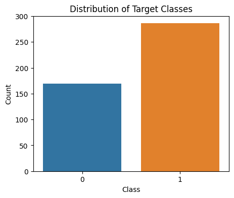
Target class distribution of SKlearn breast cancer dataset

This will help us to understand the class distribution of of the target variable. Here our target variable has two classes that are Malignant and Benign. The bincount function in NumPy is used in this code to count the samples in each class of the training data. The distribution of the target classes is then depicted in a bar plot using Seaborn, with class labels on the x-axis and class counts on the y-axis.

Correlation Matrix

For plotting a correlation matrix , first of all we will be converting the data into dataframe as dataset being a 1-Dimensional and due to that correlation matrix cannot be plotted.

Converting data to datafrome

Python3

# Set the correlation threshold
threshold = -0.4  # Adjust this threshold as needed

# CONVERT TO PANDAS DATAFRAME
df = data.frame

# Calculate the correlation matrix
correlation_matrix = df.corr()

#correlation_matrix[correlation_matrix['target'] > threshold]
index = correlation_matrix[correlation_matrix['target']> threshold].index

The code creates a correlation matrix for a pandas DataFrame df, finds columns that have a correlation higher than a given threshold with a “target” column, and then computes a correlation matrix for only those selected columns, effectively filtering for high-correlation relationships.

Plotting Correlation Matrix

Python3

# Filter the columns with correlation above the threshold for 'target'
selected_columns = correlation_matrix[correlation_matrix['target']
                                      > threshold].index

# Create a subset DataFrame with only the selected columns
correlation_matrix_filtered = df[selected_columns].corr()

# Create a heatmap to visualize the filtered correlation matrix
plt.figure(figsize=(8, 4))
sns.heatmap(correlation_matrix_filtered, annot=True,
            cmap="coolwarm", fmt=".1f", linewidths=0.1)
plt.title("Correlation Matrix for Columns with Correlation > {}".format(threshold))
plt.show()

Output:

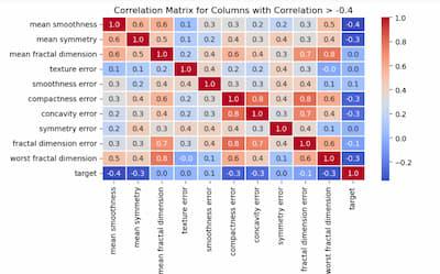
Correlation Matrix

A correlation matrix’s columns with a correlation with the ‘target’ column above a given threshold are initially identified by this code. In order to make it easier to study high-correlation associations with the “target,” it then constructs a subset DataFrame comprising only those chosen columns and generates a heatmap to illustrate the correlation matrix of those filtered columns.

Creating LightGBM dataset

To train a model using LightGBM, we need to perform this extra step. The raw dataset can’t be feed directly to the LightGBM as it has its own dataset format which is very much different from traditional NumPy arrays or Pandas Data Frames. This special data format is used for optimized internal processes during training phase.

Python3

# Create LightGBM datasets for training and testing
train_data = lgb.Dataset(X_train, label=y_train)
test_data = lgb.Dataset(X_test, label=y_test, reference=train_data)

The data are prepared for a LightGBM model’s training by this code. In order to guarantee consistent feature mapping throughout model assessment, it builds LightGBM datasets for both the training and testing sets, linking the testing dataset with the reference of the training dataset.

Model training

Python3

# Define hyperparameters
params = {
    "objective": "binary",
    "boosting_type": "rf",
    "num_leaves": 5,
    "force_row_wise": True,
    "learning_rate": 0.5,
    "metric": "binary_logloss",
    "bagging_fraction": 0.8,
    "feature_fraction": 0.8
}
# Train the LightGBM model
num_round = 500
bst = lgb.train(params, train_data, num_round, valid_sets=[test_data])

Output:

[LightGBM] [Info] Number of positive: 286, number of negative: 169
[LightGBM] [Info] Total Bins 4548
[LightGBM] [Info] Number of data points in the train set: 455, number of used features: 30
[LightGBM] [Info] [binary:BoostFromScore]: pavg=0.628571 -> initscore=0.526093
[LightGBM] [Info] Start training from score 0.526093

Now we will train the Binary classification model using LightGBM. For this we need to define various hyperparameters of the LightGBM model which are listed below:

• objective: This parameter specifies the type of task we are performing which is set to “binary” here because we are working on a binary classification problem (malignant or benign).
• boosting_type: The type of Boosting. By default it is ‘gbdt’ and also have ‘rf’ and ‘dart’ variations. Here we will use random forest boosting type i.e. ‘rf’.
• num_leaves: The number of leaves present in each tree which controls the complexity of the trees in the ensemble. Setting it very small may lead to underfitting problem.
• force_row_wise: When this is set to ‘True’ then it enables the row-wise histogram optimization mode. This can be useful for efficient training with large datasets. It is suggested to set true otherwise by default LightGBM will attempt to do it which may lead to extra overhead training time.
• learning_rate: The learning rate controls the step size during gradient boosting. It’s a value between 0 and 1. Lower values make the learning process more gradual which potentially improves generalization.
• metric: This parameter specifies the evaluation metric to monitor during training. As we are performing binary classification task, we will set it to “binary_logloss” which is the binary logarithmic loss (log loss) metric.
• bagging_fraction: The fraction of data which is randomly selected for bagging (bootstrapping). It controls the randomness in the training process and helps to prevent overfitting.
• feature_fraction: The fraction of features which is randomly selected for each boosting round. Like bagging, it introduces randomness to improve model robustness and reduce overfitting.
• num_round: The total number of boosting rounds (trees) to train.

Model Evaluation

Now we will evaluate our model based on model evaluation metrics like accuracy, precision, recall and F1-score.

Python3

# Make predictions
y_pred = bst.predict(X_test)

# Convert probabilities to binary predictions
y_pred_binary = (y_pred > 0.5).astype(int)

# Evaluate model
accuracy = accuracy_score(y_test, y_pred_binary)
precision = precision_score(y_test, y_pred_binary)
recall = recall_score(y_test, y_pred_binary)
f1score = f1_score(y_test, y_pred_binary)
# Print metrics
print(f"Accuracy: {accuracy:.4f}")
print(f"Precision: {precision:.4f}")
print(f"Recall: {recall:.4f}")
print(f"F1-Score: {f1score:.4f}")

Output:

 Accuracy: 0.9561
Precision: 0.9583
Recall: 0.9718
F1-Score: 0.9650

This code initially uses the test data to create predictions using a LightGBM model (assumed to be stored in the bst variable). Then, using a threshold of 0.5, it turns these anticipated probabilities into binary predictions. It then assesses the model’s performance based on standard classification measures like accuracy, precision, recall, and F1-score and outputs the findings.

Classification Report

Python3

# Generate classification report
report = classification_report(y_test, y_pred_binary)
print("Classification Report:\n", report)

Output:

Classification Report:
               precision    recall  f1-score   support
           0       0.95      0.93      0.94        43
           1       0.96      0.97      0.97        71
    accuracy                           0.96       114
   macro avg       0.96      0.95      0.95       114
weighted avg       0.96      0.96      0.96       114

With the help of this code, a classification report for a test dataset’s predictions from a machine learning model is produced. Each class in the target variable is given a full overview of several classification metrics in the report, including precision, recall, F1-score, and support.

Conclusion

In conclusion, using LightGBM to conduct binary classification tasks has shown to be a highly effective way to improve model performance. The 95.61% accuracy and remarkable 96.50% F1-score gained show how effective LightGBM is at enhancing model accuracy and precision. Despite the extraordinary nature of these results, it’s vital to keep in mind that accuracy may be significantly lower in real-world circumstances with larger datasets. In spite of this, the general trend shows that LightGBM can be a potent tool for improving model performance, making it a worthwhile option for a variety of machine learning applications, particularly when working with complicated and high-dimensional data. For large-scale applications where model accuracy and speed are essential components, its speed and efficiency make it particularly ideal.