LightGBM Leaf-wise Tree Growth Strategy

When it comes to machine learning and data analysis, decision trees are a fundamental tool used for classification and regression tasks. LightGBM is a popular gradient-boosting framework that employs an innovative tree growth strategy known as “leaf-wise” growth. One of the key features of LightGBM is its leaf-wise tree growth strategy, which differs from the conventional level-wise tree growth strategy used by most other decision tree learning algorithms.

In this article, we will explain what is the leaf-wise tree growth strategy and how this strategy is different from the traditional level-wise tree growth strategy used by most other decision tree learning algorithms.

What is LightGBM?

LightGBM (Light Gradient Boosting Machine) is an open-source developed by Microsoft. It is widely used in the field of data science. It is a distributed, high-performance gradient boosting framework for machine learning. It is designed to efficiently train large datasets and build highly accurate predictive models.

Before we dive into leaf-wise tree growth, let’s define some essential terminologies:

• Gradient Boosting: A machine learning technique that combines multiple weak models (usually decision trees) to create a strong predictive model.
• Decision Tree: A tree-like model that makes decisions based on features at each internal node and assigns labels at the leaf nodes.
• LightGBM: A gradient boosting framework developed by Microsoft that efficiently trains decision trees for various machine learning tasks.

Traditional Depth-wise Tree Growth

Understanding the conventional depth-wise tree growth approach used in decision trees and many other gradient-boosting frameworks is crucial to comprehending Leaf-wise development. The tree splits horizontally at each level during depth-wise growth, resulting in a wider and shallower tree. The most typical method for developing decision trees in gradient boosting is the level-wise tree development technique. Before going to the next level of the tree, it expands every node at the same level (depth). The best feature and threshold that optimizes the goal function divides the root node into two child nodes. Then, until a stopping requirement is satisfied (such as maximum depth, minimum number of samples, or minimal improvement), the same procedure is repeated for each child node. The level-wise tree growth approach makes sure the tree is balanced and that all of the leaves have the same depth.

Leaf-wise Tree Growth

Leaf-wise Tree Growth is an alternate method for developing decision trees in gradient boosting is the leaf-wise tree growth approach.

It operates by enlarging the leaf node with the biggest split gain out of all the tree’s leaves. The best feature and threshold that optimize the goal function divides the root node into two child nodes. The procedure is then repeated until a stopping condition (such as maximum depth, maximum number of leaves, or minimum improvement) is reached by choosing one of the child nodes as the next leaf to split. Even using a leaf-wise tree development plan, the tree may not be balanced or have leaves of similar depth.

In contrast to depth-wise growth, LightGBM uses leaf-wise growth. In this approach, the algorithm chooses the leaf node that provides the greatest loss function decrease, resulting in a deeper and narrower tree. Compared to depth-wise growth, this method can produce a model that is more accurate while having fewer nodes.

Criteria	Traditional Depth-wise Tree Growth	Leaf-wise Tree Growth
Order of expansion	Expands the tree level by level, i.e., splits all the nodes in the same level before moving to the next level.	Expands the tree leaf by leaf, i.e., splits the node with the largest split gain first, regardless of its depth.
Loss reduction	May not reduce the loss as much as possible, since it does not consider the global optimal split point.	It can reduce the loss more than depth-wise tree growth since it always chooses the most optimal split point.
Overfitting	May not overfit as much as leaf-wise tree growth, since it grows more balanced and shallow trees.	May overfit more than depth-wise tree growth, since it grows more complex and deep trees.
Complexity control	Can control the complexity of the tree by setting a limit on the maximum depth or the minimum number of samples per node.	Can control the complexity of the tree by setting a limit on the maximum number of leaves or the minimum split gain.
Examples of algorithms	C4.5, CART, XGBoost	LightGBM

Why Leaf-wise Tree Growth Strategy?

Leaf-wise tree growth strategy can improve the performance of LightGBM in terms of accuracy and efficiency. Here are some reasons why:

• Leaf-wise tree growth strategy can reduce the loss more than level-wise tree growth strategy, because it always chooses the leaf with the maximum split gain to split, which means it can find the most optimal split point at each iteration.
• Because it may restrict the complexity of the tree by limiting the number of leaves or the minimum split gain, the leaf-wise tree growth approach can prevent overfitting better than the level-wise tree growth technique. This means it can stop developing the tree when there is no appreciable improvement.
• Because fewer data instances must be scanned during each iteration, the leaf-wise tree growth technique can speed up training more quickly than the level-wise tree growth strategy. This helps conserve memory and processing resources.

Code Implementation

Now, let’s consider an example to demonstrate the effectiveness of Leaf-wise tree growth in LightGBM.

Install LightGBM

Ensure you have LightGBM installed on your system. You can use pip for this:

!pip install lightgbm

Implementation using Synthetic Data

To demonstrate the Leaf-wise tree development approach used by LightGBM in this example, a synthetic dataset will be created. To comprehend how this tactic works, we shall picture the tree’s development at each stage.

Step 1: Generate a Synthetic Dataset

We will create a simple synthetic dataset with two features and a binary target variable. The dataset will consist of 100 data points.

Python

import numpy as np
import pandas as pd
import matplotlib.pyplot as plt
import seaborn as sns  # Added seaborn for data visualization

# Generate synthetic data
np.random.seed(42)
X = np.random.rand(100, 2)
y = (X[:, 0] + X[:, 1] > 1).astype(int)

# Plot the data
sns.pairplot(pd.DataFrame({'Feature 1': X[:, 0], 'Feature 2': X[:, 1], 'Target': y}))
plt.show()

Output:

Step 2: Import LightGBM and Create a Dataset

Import LightGBM and prepare the dataset.

Python

import lightgbm as lgb

# Create a dataset
train_data = lgb.Dataset(X, label=y)

Step 3: Set Parameters and Train the Model

Configure LightGBM with Leaf-wise growth parameters and train the model.

Python

params = {
    'boosting_type': 'gbdt',
    'num_leaves': 31,
    'objective': 'binary',
}

model = lgb.train(params, train_data, 100)

Output:

[LightGBM] [Info] Number of positive: 43, number of negative: 57
[LightGBM] [Warning] Auto-choosing col-wise multi-threading, the overhead of testing was 0.123995 seconds.
You can set `force_col_wise=true` to remove the overhead.
[LightGBM] [Info] Total Bins 70
[LightGBM] [Info] Number of data points in the train set: 100, number of used features: 2
[LightGBM] [Info] [binary:BoostFromScore]: pavg=0.430000 -> initscore=-0.281851
[LightGBM] [Info] Start training from score -0.281851
[LightGBM] [Warning] No further splits with positive gain, best gain: -inf
[LightGBM] [Warning] No further splits with positive gain, best gain: -inf
[LightGBM] [Warning] No further splits with positive gain, best gain: -inf
[LightGBM] [Warning] No further splits with positive gain, best gain: -inf......

Step 4: Visualize Tree Growth

To visualize the growth of the tree, we can use plot_tree from LightGBM.

Python

import graphviz

lgb.create_tree_digraph(model, tree_index=0)

Output:

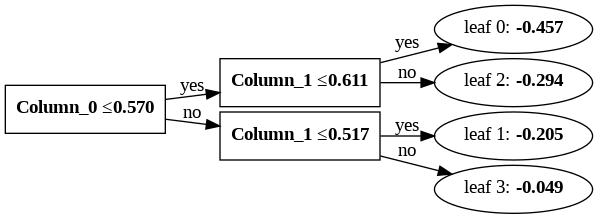
At this point, we will visualize the first tree in the model. You will notice that the tree grows deeper and narrower, optimizing the splits to reduce the loss effectively.

Implementation using Iris Dataset

We will use a publicly available dataset to demonstrate LightGBM’s Leaf-wise tree growth.

Step 1: Load a Real-World Dataset

We will use the famous Iris dataset, which contains three classes of iris plants with four features. We will visualize the tree growth for a classification task.

Python

import pandas as pd
from sklearn.datasets import load_iris
import lightgbm as lgb

# Load the Iris dataset
data = load_iris()
X = pd.DataFrame(data.data, columns=data.feature_names)
y = data.target

Step 2: Create a Dataset and Set Parameters

Prepare the dataset and set LightGBM parameters for classification.

Python

# Create a dataset
train_data = lgb.Dataset(X, label=y)

# Parameters for classification
params = {
    'boosting_type': 'gbdt',
    'num_leaves': 31,
    'objective': 'multiclass',
    'num_class': 3,
}

Step 3: Train the Model

Train the model using the dataset and parameters.

Python

model = lgb.train(params, train_data, 100)

Output:

[LightGBM] [Warning] Found whitespace in feature_names, replace with underlines
[LightGBM] [Warning] Auto-choosing col-wise multi-threading, the overhead of testing was 0.000022 seconds.
You can set `force_col_wise=true` to remove the overhead.
[LightGBM] [Info] Total Bins 98
[LightGBM] [Info] Number of data points in the train set: 150, number of used features: 4
[LightGBM] [Info] Start training from score -1.098612
[LightGBM] [Info] Start training from score -1.098612
[LightGBM] [Info] Start training from score -1.098612
[LightGBM] [Warning] No further splits with positive gain, best gain: -inf
[LightGBM] [Warning] No further splits with positive gain, best gain: -inf
[LightGBM] [Warning] No further splits with positive gain, best gain: -inf
[LightGBM] [Warning] No further splits with positive gain, best gain: -inf
[LightGBM] [Warning] No further splits with positive gain, best gain: -inf
[LightGBM] [Warning] No further splits with positive gain, best gain: -inf

Step 4: Visualize Tree Growth

Visualize the growth of a tree from the model.

Python

import graphviz

lgb.create_tree_digraph(model, tree_index=0)

Output:

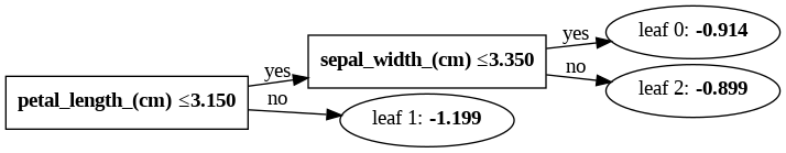
We’ll demonstrate this with the Iris dataset’s first tree from the model. To maximize splits based on information acquisition and loss minimization, the tree develops in a Leaf-wise fashion.

Now, you may learned more about LightGBM’s Leaf-wise tree development approach and how it effectively creates decision trees for diverse jobs by paying attention to these two examples and through visualizations you can understand how the tree structure changes at each stage of the procedure.

Conclusion

In this article, we have explained what leaf-wise tree growth strategy is, how it works, and why it can improve the performance of LightGBM. We have also shown an example code of using LightGBM with a leaf-wise tree growth strategy. LightGBM’s Leaf-wise tree growth strategy is a powerful technique that can help you build more accurate and efficient machine learning models. By understanding its principles and following the steps outlined in this article, you can harness the potential of this strategy for your projects. Whether you are a beginner or an experienced data scientist, LightGBM’s Leaf-wise growth is a valuable tool to have in your machine learning toolkit.