LightGBM Gradient-Based Strategy

LightGBM is a well-known high-performing model that uses a gradient-based strategy in its internal training process. Gradient-based strategy effectively enhances a model to make it highly optimized, accurate in prediction, and memory efficient which unlocks an easy way to handle complex and large real-world datasets used in various machine learning tasks. In this article, we will see the implementation of LightGBM and then visualize how its gradient-based strategy works on each feature of the dataset.

What is LightGBM

Light Gradient Boosting Machine or LightGBM is an open-source, distributed, and high-performance machine learning framework developed by Microsoft Corporation. LightGBM has gained popularity among Data Scientists as it is designed to solve large-scale classification, regression, and ranking problems which make it efficient to solve a wide range of Machine learning tasks. LightGBM utilizes a gradient-based strategy by creating an ensemble model of many decision trees which makes it a very optimized, memory-efficient, and faster algorithm.

What is a Gradient-based Strategy

Gradient-based strategy is commonly known as Gradient boosting which is a fundamental machine learning technique used by many gradient boosting algorithms like LightGBM to optimize and enhance the performance of predictive models. In a gradient-based strategy, multiple weak learners(commonly Decision trees) are combined to achieve a high-performance model. There are some key processes associated with a gradient-based strategy which are listed below:

• Gradient Descent: In the gradient-based strategy, the optimization algorithm (usually gradient descent) is used to minimize a loss function that measures the difference between predicted values and actual target values.
• Iterative Learning: The model iteratively updates its predictions for each step by calculating gradients (slopes) of the loss function with respect to the model’s parameters. These gradients are calculated to know the right way to minimize the loss.
• Boosting: In gradient boosting, weak learners (decision trees) are trained sequentially where each tree attempting to correct the errors made by the previous ones and the final prediction is the combination of predictions from all the trees.

Benefits of Gradient-based strategy

We can get several benefits in our predictive model if we utilize gradient-based strategy which are listed below:

1. Model Accuracy: Gradient boosting, including LightGBM, is known for its high predictive accuracy which is capable to capture complex relationships in the data by iteratively refining the model.
2. Robustness: The ensemble nature of gradient boosting makes it robust against overfitting problem. Each new tree focuses on the mistakes of the previous trees which reduces the risk of capturing noise in the data.
3. Flexibility: Gradient boosting has in-build mechanism to handle various types of data including both numerical and categorical features which makes it suitable for a wide range of machine learning tasks.
4. Interpretability: While ensemble models can be complex but they can offer interpretability through feature importance rankings which can be used in conjunction with interpretability tools like SHAP values to understand model decisions.

Implementation of LightGBM Gradient-Based Strategy

Installing required modules

Before implementation, we need to install LightGBM module and SHAP module which is required to visualize and explain the gradient based strategy of LightGBM.

!pip install lightgbm
!pip install shap

Importing required libraries

Python3

import lightgbm as lgb
import numpy as np
import pandas as pd
from sklearn.model_selection import train_test_split
from sklearn.metrics import mean_squared_error, mean_absolute_error, r2_score
from sklearn.datasets import load_diabetes
import matplotlib.pyplot as plt
import seaborn as sns

Now we will import all required Python libraries like NumPy, Pandas, Seaborn, Matplotlib and SKlearn etc.

Dataset loading and pre-processing

Python3

# Load the diabetes dataset from scikit-learn
diabetes = load_diabetes()
X = diabetes.data
y = diabetes.target

# Split the dataset into a training set and a testing set
X_train, X_test, y_train, y_test = train_test_split(X, y, test_size=0.2, random_state=42)

# Create a LightGBM dataset for efficient data loading
train_data = lgb.Dataset(X_train, label=y_train)
test_data = lgb.Dataset(X_test, label=y_test, reference=train_data)

We will load the Diabetes dataset of SKlearn which is dataset for regression tasks. Then we will split it into training and testing sets(80:20). One more step we need to perform which is creating LightGBM dataset by using this raw dataset. LightGBM utilizes special type of dataset loading for its internal processes which make it optimize and memory efficient.

Exploratory Data Analysis

Exploratory Data Analysis (EDA) is an essential first stage in the process of machine learning. EDA reveals data patterns, distributions, outliers, and correlations between variables by carefully analyzing the dataset. This enhanced comprehension assists with feature selection, data preparation, and model parameter tuning in addition to assisting in the selection of suitable modeling approaches. EDA serves as a compass, directing the whole modeling process to guarantee better-informed and successful model implementation.

Distribution of target feature

Visualizing distribution of variable for regression dataset is very help full to know the nature of the target or any outlier is present or not.

Python3

# Create a histogram of the target variable
plt.figure(figsize=(5, 3))
sns.histplot(y, kde=True, bins=30, color='green')
plt.xlabel('Target Variable')
plt.ylabel('Frequency')
plt.title('Distribution of Target Variable (Diabetes Dataset)')
plt.show()

Output:

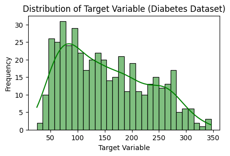
Histogram for target feature distribution

The target variable’s distribution in the Diabetes dataset is visualized using a histogram made by this code. Using a kernel density estimate (kde), it plots the histogram using the Seaborn library. Understanding the dataset’s class distribution is made easier by looking at the histogram, which shows the frequency of several target variable values.

Correlation Matrix

Visualizing the correlation matrix between features will help us to understand how features are related to each other which can give us a great understanding about the nature of whole dataset.

Python3

# Calculate and visualize the correlation matrix
correlation_matrix = np.corrcoef(X_train, rowvar=False)
plt.figure(figsize=(6, 5))
sns.heatmap(correlation_matrix, annot=True, cmap='coolwarm',
            xticklabels=diabetes.feature_names, yticklabels=diabetes.feature_names)
plt.title('Correlation Matrix')
plt.show()

Output:

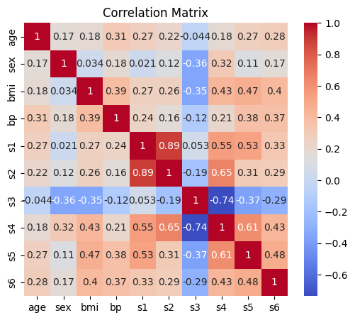
Correlation matrix for Diabetes dataset

The correlation matrix for the characteristics in the Diabetes dataset is computed and shown by this code. It uses the corrcoef function in NumPy to calculate the correlation coefficients between the features. After that, Seaborn is used to present the correlation matrix as a heatmap with annotations that highlight the strength of correlations between various characteristics, offering insights into possible feature linkages.

Model Development

Python3

# Define LightGBM parameters
params = {
    'objective': 'regression',  # Set the objective as regression
    'force_col_wise': True,
    'boosting_type': 'gbdt',   # Gradient Boosting Decision Tree
    'num_leaves': 4,         # Maximum number of leaves in one tree
    'learning_rate': 0.08,    # Learning rate (controls the step size during training)
    'min_data_in_leaf': 10,   # Minimum number of data points in a leaf
    'bagging_fraction': 0.8,  # Fraction of data used for bagging
    'feature_fraction': 0.8 # Fraction of features used for training
}

# Create a LightGBM model
model = lgb.train(params, train_data, valid_sets=[train_data], valid_names=['train'], num_boost_round=100)

Output:

[LightGBM] [Info] Total Bins 595
[LightGBM] [Info] Number of data points in the train set: 353, number of used features: 10
[LightGBM] [Info] Start training from score 153.736544

Now we will train our LightGBM model. For this we need to define different parameters which are listed below–>

1. objective: This parameter specifies the type of task we want to perform with LightGBM which is set to ‘regression’ here as we are performing regression task.
2. force_col_wise: This parameter enables column-wise histogram generation(when set to ‘True’) which is a efficient technique to handle large datasets.
3. boosting_type: This specifies the boosting type. We have set it to Gradient Boosting Decision Tree(‘gbdt’) which is a tradition way to build decision trees in a gradient boosting fashion used in gradient-based strategy.
4. num_leaves: The maximum number of leaves (terminal nodes) in each individual tree in the ensemble which set to a smaller value(4) to reduce overfitting.
5. learning_rate: It controls the step size during the training process which is set to 0.08 here. A smaller learning rate requires more boosting iterations for convergence but may result in better generalization.
6. min_data_in_leaf: It specifies the minimum number of data points required in a leaf (terminal node) of the decision tree which helps prevent the creation of very small leaves and stops overfitting.
7. bagging_fraction: It controls the fraction of data used for bagging which is a technique that involves training multiple models on random subsets of the data and then averaging their predictions and reduce overfitting.
8. feature_fraction: It is the fraction of features to be randomly selected for each boosting round which introduces randomness to improve model robustness and reduce overfitting.
9. num_round: The number of boosting rounds (trees) to train which is set to 100 i.e. 100 trees will be trained in the ensemble.

Model Evaluation

Now we will check our model’s performance based on various model performance metrics like RMSE, R2-score and MAE.

Python3

# Make predictions on the test set
y_pred = model.predict(X_test, num_iteration=model.best_iteration)

# Calculate model evaluation metrics
rmse = np.sqrt(mean_squared_error(y_test, y_pred))
mae = mean_absolute_error(y_test, y_pred)
r2 = r2_score(y_test, y_pred)
print(f'Root Mean Squared Error (RMSE): {rmse:.2f}')
print(f'Mean Absolute Error (MAE): {mae:.2f}')
print(f'R2-Score: {r2:.2f}')

Output:

Root Mean Squared Error (RMSE): 51.52
Mean Absolute Error (MAE): 40.99
R2-Score: 0.50

This code uses a trained model to make predictions on the test set. Next, the code computes the R-squared (R2), Mean Absolute Error (MAE), and Root Mean Squared Error (RMSE), three commonly used metrics for evaluating regression. By evaluating the accuracy and goodness of fit between the anticipated and actual values, these metrics offer valuable insights into the model’s performance. The outcomes can be analyzed by printing them to the console.

Gradient-based strategy visualization

Now we will SHAP module to see how the features of the dataset is used in the model’s decision-making process which provides a clear and intuitive representation of the distribution of SHAP values for each feature and allows us to see the spread of feature effects and their impact on predictions.

Python3

import shap
# Create a SHAP explainer for the LightGBM model
explainer = shap.Explainer(model)

# Calculate SHAP values for a specific instance or dataset
shap_values = explainer.shap_values(X_test)

# Plot a summary plot of SHAP values
shap.summary_plot(shap_values, X_test, plot_type="violin", plot_size= 0.2,feature_names=diabetes.feature_names)

Output:

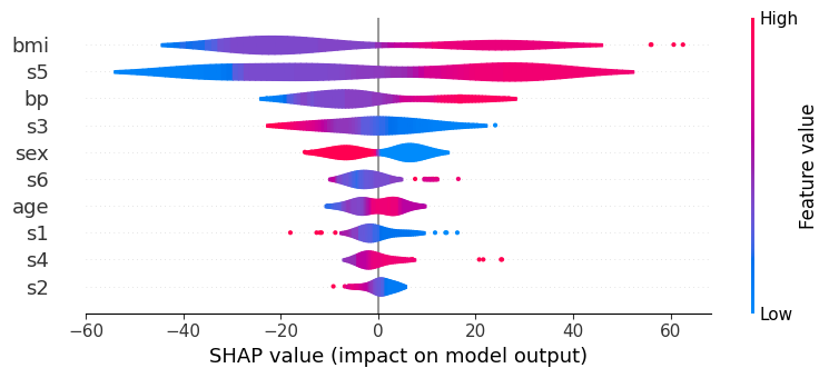
Model’s gradient-based strategy visualization

This code makes use of the SHAP (SHapley Additive exPlanations) package to offer explanations for the predictions generated by a LightGBM model. We may comprehend the significance of individual aspects in the predictions by using the explainer for the model that is created using the shap.Explainer. For the test dataset, SHAP values are calculated to show how each feature affects the model’s output. A summary plot in the style of violin plots is then used to show these values, providing a clear picture of how each feature affects the model’s predictions and assisting in the interpretation and decision-making process.

Conclusion

We can conclude that, gradient-based strategy is an effective technique to handle large datasets, utilize memory and optimize training processes. LightGBM utilizes gradient-based mechanism which makes it a powerful machine leaning model. Here, our model achieved well performance with less values of error metrics and moderately good R-score of 50%. However, in real-world dataset this performance may be more degraded so fine-tuning is required in that case.