How to use TensorBoard in Google Colab?

TensorBoard is indeed an invaluable tool. It serves as a comprehensive visualization toolkit with the TensorFlow ecosystem, enabling practitioners to experiment, fine-tune, and monitor, the training of machine learning models with ease. By offering a dynamic and intuitive dashboard, TensorBoard allows users to gain a deeper understanding of their model’s behaviour and performance.

TensorBoard

The dashboard for TensorBoard provides a wide range of visualization choices, such as graphical depictions of training and validation metrics, data images, histograms showing parameter distributions, and embeddings that assist in visualizing high-dimensional data in lower dimensions. This comprehensive toolbox equips academics and industry professionals to solve problems efficiently, optimize model designs, and make data-driven decisions.

Installation

It is pre-built in Google Colab. If you want to use it on your system, you can install it by:

pip install tensorflow

pip install tensorboard

The above command helps you to install TensorFlow and TensorBoard respectively.

Uses of TensorBoard

TensorBoard has different uses in ML experimentation and a few are given below:

1. Track and Visualise Metrics (Loss & accuracy): Use tf.keras.callbacks.TensorBoard to visualise loss and accuracy matrices. It is used to create an interactive visualisation and track the progress of model training.
2. Visualize Operations and Layers Graph: It is used to visualise the training of layers and operations performed on the same i.e. to visualise the architecture of the model. It may be done by tf.keras.utils.plot_model.
3. Viewing histograms and tracking changes over time: You have ‘histogram’ functionality in the tensor board which can be called using tf.summary.histogram. It helps to visualise the log of weights, biases or any other tensor in the model.
4. Projecting Embeddings to Lower Dimensional Space: It supports audio files, images and text files which can be logged using ‘tf.summary.image’, ‘tf.summary.audio’, and ‘tf.summary.text’ for image, audio, and text file respectively.
5. Profiling Programs: Use tf.profiler to identify the bottleneck in the TensorFlow program. It is also used to view the time and memory consumption of the code in different operations.

Running Tensorboard in Google Colab

To run TensorBoard on Colab, we need to load tensorboard extension. Run the following command to get tensor board extension in Colab:

• This helps you to load the tensor board extension. Now, it is a good habit to clear the pervious logs before you start to execute your own model.

%load_ext tensorboard

• Use the following code to clear the logs in Colab:

!rm -rf ./logs/

• Now, we want a callback so we need to add a folder where we want to save the logs. You may do it with the following command:

log_dir = "myLogs/Logs/" + datetime.datetime.now().strftime("%d-%m-%Y-%H%M%S") #You may add your own directory

• We shall do a callback to tensor board. The following code is helpful (for model train metrics):

tensorboard_callback = tf.keras.callbacks.TensorBoard(log_dir=log_dir, histogram_freq=1)

As we have discussed the basis of model, We will present a way to execute it in Google Colab. You may paste code cell by cell and run to see the output.

Python3

%load_ext tensorboard  #loads tensorboard
!rm -rf ./myLogs/ #removes the log folder

It will load the tensor board. In case, if you want to reload it run ‘%reload_ext tensorboard’.

Building a TensorBoard

Now we fetch MNIST dataset and create our own model by the following piece of code:

Installing Libraries

Python3

#installing necessary libraries
import tensorflow as tf
import datetime
from tensorflow import keras

Here , we are installing necessary libraries to make our model work.

Loading and splitting train test dataset

Python3

#Load MNIST dataset
mnist = tf.keras.datasets.mnist
#Create test train split
(x_train, y_train),(x_test, y_test) = mnist.load_data()
x_train, x_test = x_train / 255.0, x_test / 255.0

Here , we are loading the dataset and splitting the data set into train and test dataset.

Building the Model

Python3

# Write your TF Model
model = keras.Sequential()
model.add(keras.layers.Conv2D(input_shape=(28, 28, 1), filters=8,
                              kernel_size=3, strides=2, activation='relu', name='Conv1'))
model.add(keras.layers.Conv2D(filters=16, kernel_size=3,
                              activation='relu', name='Conv2'))
model.add(keras.layers.MaxPooling2D(pool_size=(2, 2), name='MaxPool1'))
model.add(keras.layers.Conv2D(filters=32, kernel_size=3,
                              activation='relu', name='Conv3'))
model.add(keras.layers.Flatten())
model.add(keras.layers.Dense(64, activation='relu', name='Dense1'))
model.add(keras.layers.Dense(32, activation='relu', name='Dense2'))
model.add(keras.layers.Dense(10, name='Dense3'))
# Get model summary
model.summary()

Output:

Downloading data from https://storage.googleapis.com/tensorflow/tf-keras-datasets/mnist.npz
11490434/11490434 [==============================] - 0s 0us/step
Model: "sequential"
_________________________________________________________________
 Layer (type)                Output Shape              Param #   
=================================================================
 Conv1 (Conv2D)              (None, 13, 13, 8)         80        
                                                                 
 Conv2 (Conv2D)              (None, 11, 11, 16)        1168      
                                                                 
 MaxPool1 (MaxPooling2D)     (None, 5, 5, 16)          0         
                                                                 
 Conv3 (Conv2D)              (None, 3, 3, 32)          4640      
                                                                 
 flatten (Flatten)           (None, 288)               0         
                                                                 
 Dense1 (Dense)              (None, 64)                18496     
                                                                 
 Dense2 (Dense)              (None, 32)                2080      
                                                                 
 Dense3 (Dense)              (None, 10)                330       
                                                                 
=================================================================
Total params: 26794 (104.66 KB)
Trainable params: 26794 (104.66 KB)
Non-trainable params: 0 (0.00 Byte)
_________________________________________________________________

This code defines a CNN model using Tensorflow’s Keras API. It consists of three convolutional layers(conv2D), followed by max-pooling and fully connected layers(Dense). The model’s input shape is (28,28,1), suitable for grayscale images, and it ends with an output layer with 10 units for classification. The ‘model_summary()’ function is used to display a summary of the model’s architecture, including layer names, output shapes, and the total number of parameters.

Before training Load the tensorboard and clear the log folder

Python3

# Load the tensorboard
%load_ext tensorboard
#removes the log folder
!rm -rf ./myLogs/

Training the model

Now we train model with tensor board callback:

Python3

#Compie Model
model.compile(optimizer='adam',
              loss='sparse_categorical_crossentropy',
              metrics=['accuracy'])

#Create directory to store logs
log_ = "myLogs/modelFit/" + datetime.datetime.now().strftime("%d-%m-%Y-%H%M%S")
#Tendorboard call backs
tensorboard_callback = tf.keras.callbacks.TensorBoard(log_dir=log_, histogram_freq=1)
#Train the mdel with tensorboard callback
model.fit(x=x_train,
          y=y_train,
          epochs=10,
          validation_data=(x_test, y_test),
          callbacks=[tensorboard_callback])

Output:

Epoch 1/10
1875/1875 [==============================] - 21s 5ms/step - loss: 2.3364 - accuracy: 0.0980 - val_loss: 2.3026 - val_accuracy: 0.0988
Epoch 2/10
1875/1875 [==============================] - 8s 4ms/step - loss: 2.3026 - accuracy: 0.0965 - val_loss: 2.3026 - val_accuracy: 0.0988
Epoch 3/10
1875/1875 [==============================] - 8s 4ms/step - loss: 2.3026 - accuracy: 0.0965 - val_loss: 2.3026 - val_accuracy: 0.0988
Epoch 4/10
1875/1875 [==============================] - 8s 5ms/step - loss: 2.3026 - accuracy: 0.0965 - val_loss: 2.3026 - val_accuracy: 0.0988
Epoch 5/10
1875/1875 [==============================] - 11s 6ms/step - loss: 2.3026 - accuracy: 0.0965 - val_loss: 2.3026 - val_accuracy: 0.0988
Epoch 6/10
1875/1875 [==============================] - 8s 4ms/step - loss: 2.3026 - accuracy: 0.0965 - val_loss: 2.3026 - val_accuracy: 0.0988
Epoch 7/10
1875/1875 [==============================] - 9s 5ms/step - loss: 2.3026 - accuracy: 0.0965 - val_loss: 2.3026 - val_accuracy: 0.0988
Epoch 8/10
1875/1875 [==============================] - 8s 4ms/step - loss: 2.3026 - accuracy: 0.0965 - val_loss: 2.3026 - val_accuracy: 0.0988
Epoch 9/10
1875/1875 [==============================] - 8s 4ms/step - loss: 2.3026 - accuracy: 0.0965 - val_loss: 2.3026 - val_accuracy: 0.0988
Epoch 10/10
1875/1875 [==============================] - 8s 5ms/step - loss: 2.3026 - accuracy: 0.0965 - val_loss: 2.3026 - val_accuracy: 0.0988
<keras.src.callbacks.History at 0x7ed29ff39e40>

Here , this code compiles a previously defined Keras model using Adam optimizer, sparse categorical cross-entropy loss function, and accuracy as the evaluation metric. It then creates a directory for storing training logs with a timestamp. The ‘tensorboard_callback’ is setup to enable tensorboard logging. Finally the model is trained using the training data for 10 epochs while validating on the test data. The TensorBoard callback is used to log training progress for later analysis and visualization.

Log File Folder

As we have trained the model, we may see the hierarchy of folder created with log files in the runtime of Google Colab as shown below:

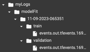
Fig: Logs

Since, we created the logs, and trained the model, we may visualize it by:

%tensorboard --logdir <your log folder>

Here , the ‘%tensorboard’ command is used to call the Tensorboard extension. The ‘–logdir’ parameter specifies the directory where the model training logs are stored, allowing users to easily visualize and interact with the training progress and metrics using Tensorboard’s web interface. This enables user to gain insights into the model performance, loss trends, and other information during training. In our case, we may do it by:

Python3

%tensorboard --logdir myLogs/modelFit/

It will display tensor board in an interactive window as shown below:

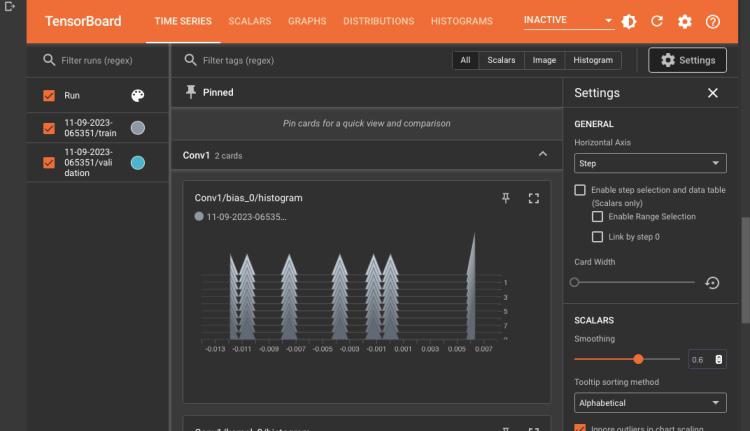
Tensorboard

This is how you use TensorBoard in Google Colab.

Conclusion

In conclusion, TensorBoard is a vital tool for machine learning and deep learning, offering a wide range of options for managing experiments, visualizing models, and keeping track of results. This post has emphasized its importance and shown how it may be applied practically in the Google Colab setting.

The dynamic and user-friendly interface of TensorBoard offers a variety of visualization choices, such as graphical representations of training metrics, parameter distributions, and high-dimensional data projections, allowing users to get deeper insights into the behavior and performance of their models. These capabilities give academics and business experts the tools they need to solve issues quickly, improve model architectures, and reach data-driven conclusions.Users may set up their environments without difficulty because to the well described installation procedure for TensorFlow and TensorBoard. The paper also included instructions on how to load and clean logs and a step-by-step walkthrough for creating and training a model while utilizing TensorBoard for analysis and monitoring.