How to Highlight Duplicates in Google Sheet

Explore the world of Google Sheets and get into the art of highlighting duplicates in Google Sheets. Whether you’re a spreadsheet pro or just a newbie in the data-driven field, understanding how to spot and find duplicate values can enhance your productivity and accuracy. In this journey of learning different features of Google Sheets, we’ll learn the secrets behind conditional formatting, learn the UNIQUE function, and even venture into multiple columns.

Why Highlight Duplicates in Google Sheets?

If you have a table or a row where you might accidentally enter the same information(like a name, a product, or a date) more than once. These are duplicates in Google Sheets. Identifying duplicates or highlighting duplicates in Google Sheets is important because Duplicates can mess up your data. So, by finding these, you can keep your data accurate, efficient, and more organized.

What Found a Duplicate in a Dataset

In a Google Sheet, a duplicate refers to a data entry that appears more than once, meaning there are identical or similar records present for a particular entity or observation. Here’s an explanation like,

• Identical Entries
• Similar Entries
• Unique Identifiers
• Contextual Relevance
• Duplicates Across Multiple Columns

How to Highlight Duplicates in Google Sheets

Highlighting duplicates in Google Sheets is a straightforward process, where users can easily spot duplicates using a conditional formatting process. Here’s the step-by-step guide provided below for you all,

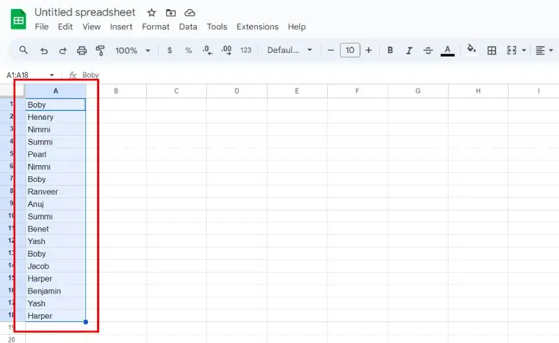
Step 1: Select the cell

Select the range of cells where you want to identify duplicates.

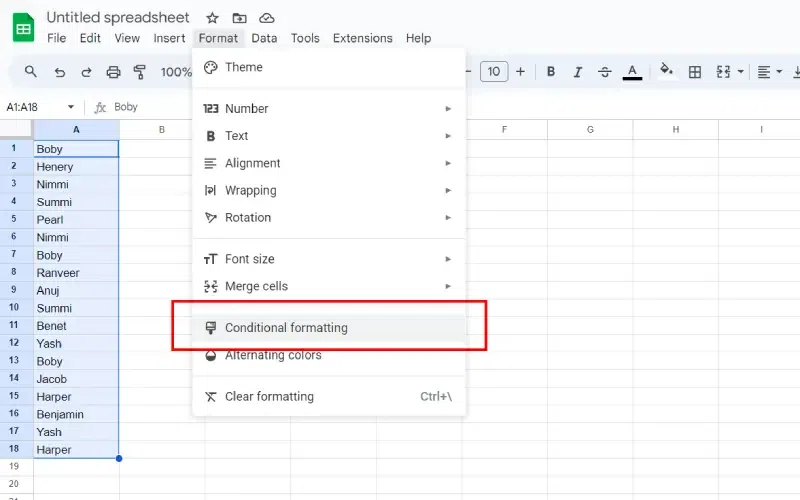
Step 2: Click on ‘Format’

Navigate through the menu bar and click on “Format” in the menu bar.

Step3: Choose ‘Conditional Formatting’

In the format option, go to “Conditional formatting.”

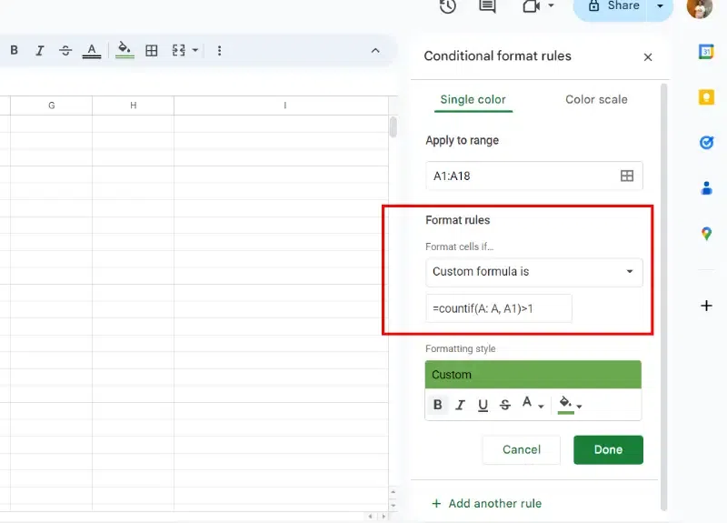
Step 4: Choose ‘Custom formula is’

In the conditional formatting rules, choose “Custom formula is” from the drop-down menu.

Step 5: Enter the Formula and choose a style

Enter the formula to identify duplicates, such as

“=countif(A: A, A1)>1”

(assuming your data is in column A). Choose the formatting style for highlighting duplicates, like a different background color or text color.

Step 6: Click ‘Done’

Click “Done” to apply the formatting in the cells.

Highlight Duplicates in Multiple Rows and Columns

Step 1: Select the Range

Click and drag to select the range of cells where you want to highlight duplicates.

Step 2: Open Conditional Formatting

Go to the “Format” menu, then select “Conditional formatting.”

Step 3: Set Up the Rule

In the conditional formatting pane, choose “Custom formula is” from the dropdown.

Step 4: Enter the following formula

=COUNTIF($A$1:$Z$100,A1)>1

This formula assumes your range goes from A1 to Z100. Adjust it based on your actual range. It checks if the current cell has duplicates in the selected range.

Step 5: Choose Formatting

Click on the paint bucket icon to choose the formatting style for highlighting duplicates. You can select a background color, text color, or any other formatting you prefer.

Step 6: Apply

Click “Done” to apply the conditional formatting.

Conclusion

In the end, checking and highlighting duplicates in Google Sheets is a normal process, anybody can try this by using a conditional formatting process. Users can quickly spot the difference or duplicate entries by applying custom formulas. It makes analysis and data management more efficient. This feature enhances the usability of Google Sheets and users can make an organized Sheets for effective data interpretation and decision-making.

FAQs – Highlight and Remove Duplicates in Google Sheets

Can you highlight duplicates in Google Sheets?

Yes, In Google Sheets you can easily highlight Duplicates and filter them out.

Is there a way to filter duplicates in Google Sheets?

• Select the range of cells where you want to check for duplicates.
• Go to the menu at the top and click on “Format.”
• Choose “Conditional formatting.”
• In the sidebar that appears on the right, under the “Format cells if” dropdown, select “Custom formula is.”
• In the field next to it, enter the formula =COUNTIF(A: A, A1)>1 (replace A: A with the column range you’re checking, and A1 with the first cell of your selection).
• Choose the formatting style you want for the duplicates, like background color or text color.
• Click “Done.”

Is there a way to highlight duplicates?

• Select the range of cells containing your data.
• Go to the menu at the top and click on “Data.”
• Choose “Filter.”
• Click the dropdown arrow on the column header you want to filter.
• Choose “Filter by condition.”
• Select “Duplicate.”
• Google Sheets will show you only the rows with duplicate values in that column.