How to Add Filter in Google Sheets

Adding a filter in Google Sheets helps in organizing and analyzing data more efficiently. Filters allow users to focus on specific information in your spreadsheet, which makes it easier to find what a user needs. This article will cover how to add a filter in Google Sheets, and the steps to set up filters, making your data sorting and viewing experience smoother. Also, we will see various benefits of using filters in Google Sheets.

What Are Filters in Google Sheets

Filters help you locate specific information in your Google Sheets spreadsheet. When dealing with a large amount of data, finding a particular character or value can be challenging. Filters come in handy in such situations, allowing you to set criteria for Sheets to use when searching for the information you need. This way, you can narrow down the display to show only the data you are interested in, making it more manageable.

Filters can be created based on various conditions, data points, or colors. Once applied, the filtered sheet will be visible not only to you but also to anyone with access to view your spreadsheet. This feature enables a more organized and tailored presentation of data for collaborative work or sharing information with others.

How to Filter Your Data in Google Sheets

Filters can be created both on Google Sheets web and the Google Sheets app on your phone. In this article, we will learn how to enable or add filters on the Google Sheets website. When adding a filter to your spreadsheet, keep in mind that anyone with access to the spreadsheet can see and use the filter.

Step 1: Select The Range

To initiate the process, choose a range of cells before creating the filter. To do this, open the spreadsheet in Google Sheets and manually select the cells. Begin by choosing a cell and dragging the cursor across your desired selection.

Specific Selection

To choose whole columns, click on the headers at the top. To pick multiple columns, press and hold the Ctrl or CMD key on your keyboard while selecting the columns you want.

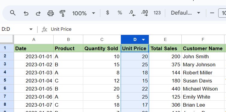
Column-Wise Selection

To choose all cells in the spreadsheet, click the rectangle at the meeting point of column A and row 1 outside the spreadsheet area.

Full-Selection

Step 2: Go to Data and Select Create Filter

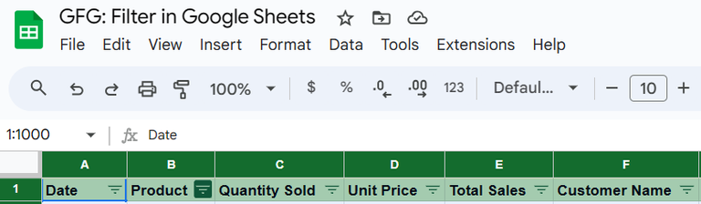
After choosing the cell range, create a filter by clicking on the Data tab in the top toolbar and then choosing Create a filter.

After this you will see the filter icons become visible at the top of the chosen columns. Customization of the filters for each column is then necessary, depending on specific requirements.

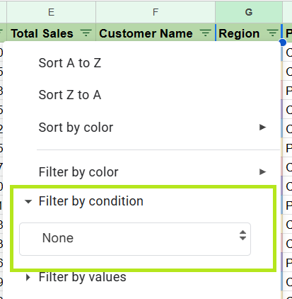
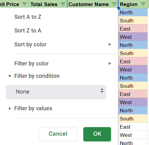
Step 3: Choose Filter by Option

Click on the filter icon, now present on the selected header of the particular column. Here, you will get three option to add filter.

• Filter by Color
• Filter by Condition
• Filter by Values

Filtering Options

How To Filter by Color in Google Sheets

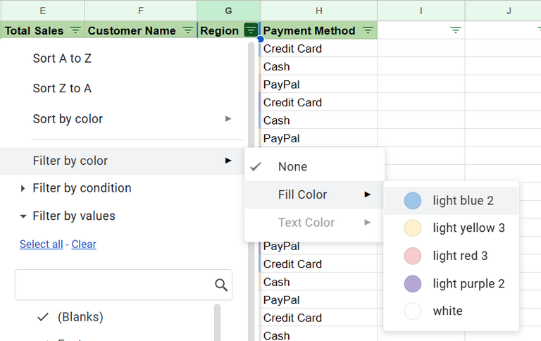
Step 1: Select Filter By Color

Choosing this option enables you to identify cells in a column distinguished by a particular color. Specify the color in Fill Color or Text Color to filter the desired data sets within the spreadsheet.

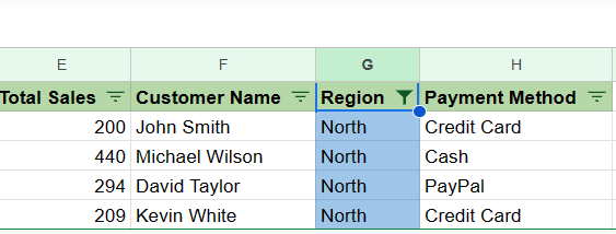
Step 2: Color Filter is Enabled

Upon selecting a color for column filtering, only rows and cells displaying the chosen color will appear in the spreadsheet.

How to Filter by Condition in Google Sheets

Step 1: Select Filter by Condition

This feature allows you to filter cells containing specific texts, numbers, dates, or formulas. It can also be used to isolate blank cells. To access additional options, click on the “Filter by condition” choice, revealing a dropdown menu where you can pick a condition. To select a condition, click on None.

Step 2: For empty cells

To filter cells with or without content, choose Is empty or Is not empty from the dropdown menu.

Step 3: For cells with texts

If dealing with text, filter the column based on criteria such as containing certain characters, starting or ending with a word/letter, or having specific words. Options include Text contains, Text does not contain, Text starts with, Text ends with, and Text is exactly. Input the desired parameters in the text box below.

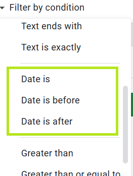
Step 4: For cells with dates

If the column has dates, filter based on Date is, Date is before, or Date is after. Choose a period or specific date from the date menu.

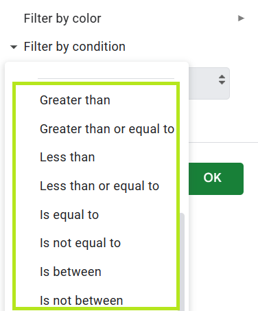
Step 5: For cells with numbers

If the cells have numbers, use criteria like Greater than, Greater than or equal to, Less than, Less than or equal to, Is equal to, Is not equal to, Is between, or Is not between. Enter desired parameters in the Value or formula box.

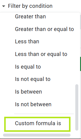
Step 6: For cells with a formula

To find cells with a specific formula, choose Custom formula is from the dropdown menu. Enter the formula in the Value or formula box.

How to Filter by Values in Google Sheets

Step 1: Select Filter by Values

To filter columns based on numbers, you can use the Filter by values option, which makes the process easier. When you choose this filtering option, you will see all the values present in the selected column cells. By default, all these values will be selected, indicating that all cells are currently visible. If you want to hide specific values from the column, simply click on them.

Step 2: Choose the Values

Depending on how many values are in the column, you can click on Select all to choose all values or Clear to hide all values. Once you have selected your desired filter, click on OK at the bottom of the Filters overflow menu.

Your spreadsheet will now be organized based on the filter you applied using the options mentioned above.

How to create and use filter views in Google Sheet from mobile

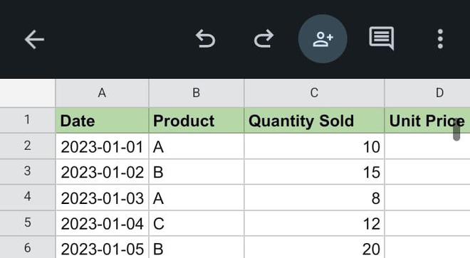
Step 1: Open Google Sheets App

Launch the Google Sheets app on your Android phone or iPhone.

Step 2: Select Spreadsheet

Choose the specific spreadsheet you wish to edit.

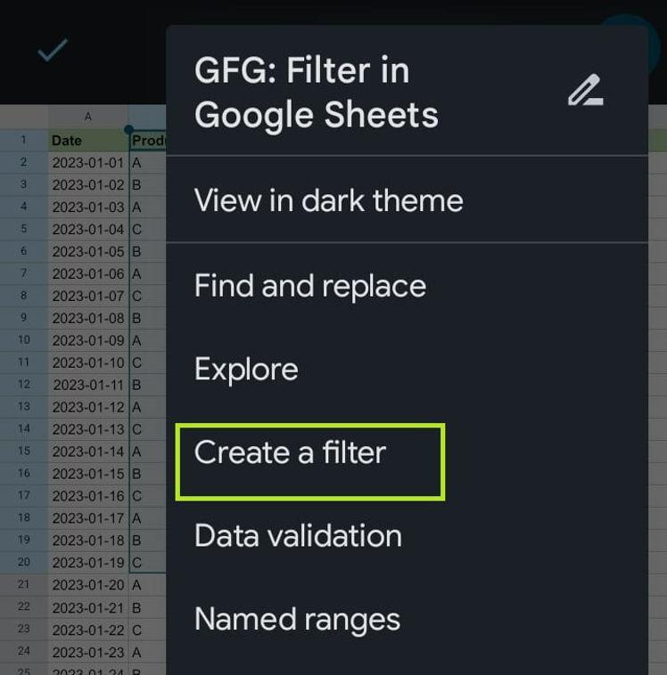
Step 3: Go to Menu Option (three dots) Icon

Once the spreadsheet is open, tap on the 3-dots icon located at the top right corner.

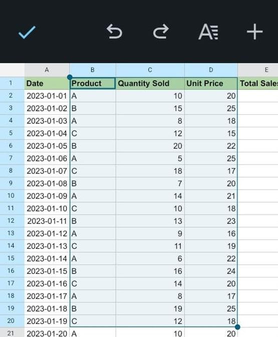
Step 4: Navigate to Filter Creation

Select the cell range option in the side bar that appears, and insert the cell range where you wish to add filter.

Again click on the three dots icon and now there will be option for Create Filter on the side bar, click on it.

Step 5: Apply Filters Across Columns

Filter icons will now be visible at the headers of all columns.

Step 6: Customize a Column’s Filter

To personalize a filter in a specific column, tap on the filter icon corresponding to that column.

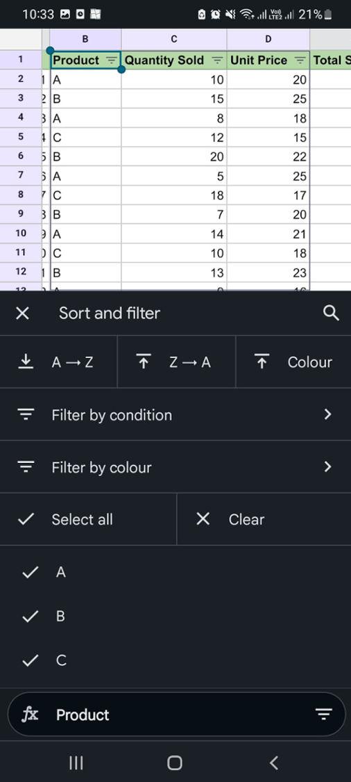
Step 7: Explore Filtering Options

• A popup box will appear at the bottom half of the screen, providing various filtering options.
• For “Filter by condition,” select criteria and add parameters.
• In “Filter by color,” opt for Fill color or Text color and choose the desired color for filtering.
• While “Filter by values” isn’t explicitly labeled, you can use it by selecting values from existing cells in the column, displayed under the “Filter by color” section.

Once you’ve customized the necessary filters, tap on the checkmark at the top left corner to confirm the changes.

Step 8: View Updated Spreadsheet

The spreadsheet will now be rearranged based on the filters you’ve applied.

Filter v/s Filter Views

Filters in a spreadsheet are essential for data analysis, but when collaborating, applying filters or sorting columns impacts everyone’s view. Users with editing rights can also modify filters, while viewers without editing access cannot use or change them. For more seamless collaboration, Google Sheets introduces Filter Views. These allow the creation of custom filters highlighting specific data without altering the original view for others. Unlike regular filters, Filter Views only affect the user’s view temporarily. They offer the flexibility to create and save multiple filter views for diverse data sets. Importantly, users with view-only access can apply and use filter views, enabling better collaboration without altering the original spreadsheet view.

How to Remove Filters From Google Sheets

To remove the filters from Google Sheets is a easy process, follow the below steps:

Step 1: Decide on Filter Removal Method

If you put a filter on a Google Sheets column and want to remove it, there are two ways: either remove specific details or completely eliminate the filter.

Step 2: Access Filter Icon

To reset a filtered column, click on the Filter icon located in the column’s header.

Step 3: Confirm Reset

A window will appear; click on OK to confirm. The column will return to its original appearance, but the filter icon will still be visible.

Step 4: Remove Filter Icon

If you want to eliminate the filter icon, go to the Data tab in the top toolbar.

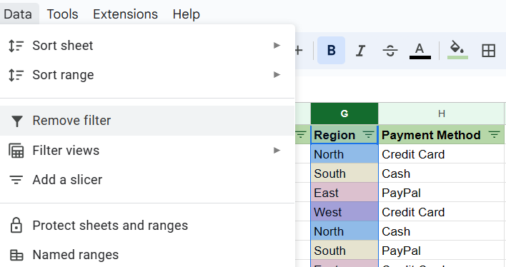
Step 5: Choose “Remove Filter”

Select “Remove filter” from the options. This action will remove filters from all columns in the spreadsheet.

Conclusion

Using filters in Google Sheets makes it easier to organize and analyze data. Filters help find specific information in large datasets, improving collaboration. Whether on the web or the mobile app, the provided steps guide users through a smooth filtering process. Understanding the benefits of filters and how they differ from Filter Views contributes to more efficient data management. Removing filters is a straightforward process, allowing for flexibility in adjusting spreadsheet views.

FAQs

How do I create a drop-down filter in Google Sheets?

To create a drop-down filter in Google Sheets, select the cell range you want to filter, click on “Data,” and choose “Create a filter.”

How do I add a filter to every column in Google Sheets?

Adding a filter to every column in Google Sheets is done by selecting any cell within the data range, clicking on “Data,” and selecting “Create a filter” to enable filters for all columns.

How do I use the filter function in Google Sheets?

To use the filter function in Google Sheets, select the data range, click on “Data,” and choose “Create a filter.” You can then customize and apply specific filters to your data.

How do I add a filter to a Google sheet chart?

Adding a filter to a Google Sheets chart is not directly possible. However, you can filter the underlying data, and the chart will dynamically update based on the filtered information.