Effect of Transforming the Targets in Regression Model

Regression modelling plays a crucial role in predicting numerical outcomes and understanding the relationships between variables. One key aspect of building robust regression models is the careful consideration of the target variable, as its distribution and characteristics can significantly impact model performance. In this article, we will discuss the effect of transforming the targets in regression modelling and their benefits.

Why Transform Targets?

We need to perform target variable transformations in real-world regression-based regression datasets to address issues like non-linearity, heteroscedasticity, and skewed distributions. These complex patterns can’t be handled by linear and low-standard tree-based regression models as they blindly assume a linear relationship between predictors and the target variable. Transformation can help to mitigate these issues and improve the model’s ability to capture complex patterns. Some of the key benefits of transforming targets for regression problems are listed below:

1. Normalization of Distributions: Transformation can convert skewed or non-normal distributions into more symmetric, normal-like distributions. This is particularly beneficial as it aligns with the assumption of normality in many statistical models.
2. Stabilization of Variances: Heteroscedasticity, where the spread of residuals varies across the range of predictors, can be addressed by transforming the target variable which helps to stabilize variances and ensures that model predictions are more consistent across the entire data range.
3. Handling Non-linearity: If the relationship between predictors and the target is nonlinear, certain transformations (e.g., logarithmic or power transformations) can help capture these nonlinear patterns which makes the relationship more amenable to regression modeling.
4. Improved Model Performance: Transformation makes betterment of model performance by facilitating a more accurate representation of underlying patterns and reducing the impact of outliers.

Transformation Methods

Now we will discuss some of the common transformation methods below:

• Log Transformation: This transformation method uses logarithmic methods to reduce the impact of large values and transform exponential growth patterns. This method is particularly useful when we are dealing with variables that exhibit exponential growth like income or population size.
• Square Root Transformation: The square root transformation is employed to stabilize variances and address right-skewed distributions which is particularly useful when the variability of the target variable increases with its mean. By taking the square root, it compress the scale of larger values more than smaller ones, mitigating the impact of outliers and promoting a more homogenous spread of values.
• Quantile Transformation: Quantile transformation maps the data to a specified distribution, often a standard normal distribution. This transformation is useful for mitigating the impact of outliers and achieving a more uniform spread of values. It works by assigning a new value to each data point based on its rank order, ensuring that the transformed values follow the desired distribution. This transformation is particularly effective when the target variable has a non-normal distribution or contains extreme values.
• Box-Cox Transformation: The Box-Cox transformation is a complex method which encompasses both logarithmic and power transformations. It is designed to handle a variety of distributions and adapt to the underlying structure of the data. The Box-Cox transformation is suitable for dealing with skewness, heteroscedasticity and other distributional issues.

Effect of Transforming the Targets in Regression Model

Importing required modules

At first, we will import all required Python modules like Pandas, Seaborn, Matplotlib and SKlearn etc.

Python3

import pandas as pd
from sklearn.model_selection import train_test_split
from sklearn.linear_model import LinearRegression
from sklearn.metrics import r2_score, mean_absolute_error
import matplotlib.pyplot as plt
from sklearn.preprocessing import QuantileTransformer
import seaborn as sns

This snippet of code analyzes a dataset using linear regression using the pandas and scikit-learn libraries in Python. The required modules are imported first, and the dataset is then read into a pandas DataFrame. The data is divided into training and testing sets, and then QuantileTransformer is used to scale the features. Using the transformed data, a linear regression model is trained, and evaluation metrics like mean absolute error and R-squared are computed. Using matplotlib and seaborn, the code ends with a visual representation of the relationship between the predicted and actual values.

Dataset loading and splitting

Python3

# Load House Prices dataset
# https://www.kaggle.com/c/house-prices-advanced-regression-techniques/data?select=train.csv
data = pd.read_csv('train.csv')

# Select features and target
X = data.drop('SalePrice', axis=1)
y = data['SalePrice']

# Handle missing values and categorical features (customize as needed)
X = X.fillna(0)  # Replace NaN values with 0 for simplicity
X = pd.get_dummies(X)

# Split the dataset
X_train, X_test, y_train, y_test = train_test_split(
    X, y, test_size=0.2, random_state=42)

Now we will load a Kaggle dataset and after handling missing values we will split the dataset into training and testing sets(80:20). This code selects the target variable (y) and features (X) from the House Prices dataset that is loaded from Kaggle. NaNs are simply replaced with 0 to handle missing values. The get_dummies function in pandas is then used to one-hot encode the categorical features.

Quantile Transformation

Python3

# Linear Regression on Original Targets
model_original = LinearRegression()
model_original.fit(X_train, y_train)
y_pred_original = model_original.predict(X_test)
# QuantileTransformer
quantile_transformer = QuantileTransformer(output_distribution='normal', random_state=42)
y_train_transformed_quantile = quantile_transformer.fit_transform(y_train.values.reshape(-1, 1)).flatten()
model_quantile = LinearRegression()
model_quantile.fit(X_train, y_train_transformed_quantile)
y_pred_quantile = model_quantile.predict(X_test)
y_pred_quantile_inverse = quantile_transformer.inverse_transform(y_pred_quantile.reshape(-1, 1)).flatten()

Here we will use Quantile transformer as we have used a dataset of sales price in which we need to bypass the effect of outliers. And for model, we will use Liner Regression model. To implement quantile transformer we have handled the randomness of transformation subsets using its ‘random_state’ parameter and the distribution of output is set to ‘normal’ by ‘output_distribution’ parameter which means that after transformation the target will follow a normal distribution.

Comparative visualization of target variable

Here we will plot the distribution of target variable for raw dataset and the distribution of target variable after Quantile transformation.

Python3

# Plot the distribution of the original target
plt.figure(figsize=(8, 4))
plt.subplot(1, 2, 1)
sns.histplot(y, bins=30, kde=True, color='green')
plt.title('Distribution of Original Target')
plt.xlabel('SalePrice')
plt.ylabel('Frequency')

# Plot the distribution after transforming the target using QuantileTransformer
plt.subplot(1, 2, 2)
sns.histplot(y_train_transformed_quantile, bins=30, kde=True, color='green')
plt.title('Distribution after Quantile Transformation')
plt.xlabel('Transformed SalePrice')
plt.ylabel('Frequency')
plt.tight_layout()
plt.show()

Output:

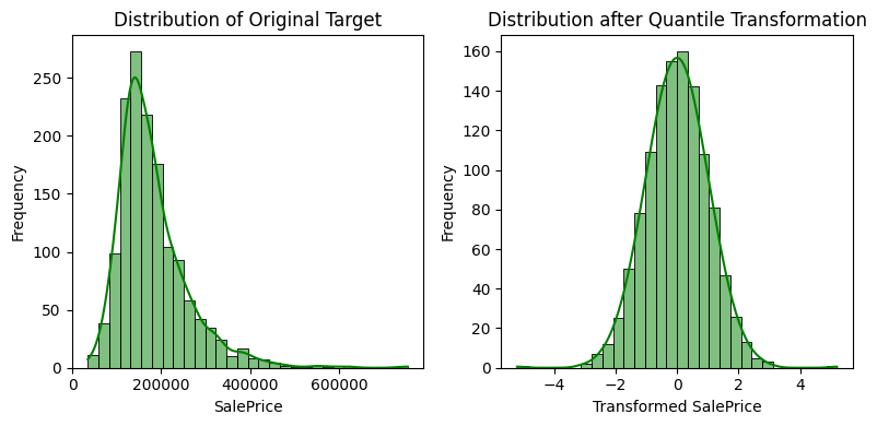
Comparative plot for raw target distribution and quantile transformed distribution

This code generates a comparison table that shows the distribution of the target variable “SalePrice” at initial values and after quantile transformation. The original target distribution is represented visually in the left subplot by a histogram with kernel density estimation. The transformed distribution is shown in the right subplot following the application of QuantileTransformer to the training set. By ensuring a more uniform distribution, the quantile transformation may help regression models that assume a normal distribution of the target variable perform better. Matplotlib and Seaborn are utilized for the visual aids.

Visualizing prediction and actual values

In this comparative plot, we will visualize the actual and predicted values for both Linear regression on raw targets and quantile transformed target.

Python3

# Plotting
plt.figure(figsize=(12, 6))

# Original Predictions vs Actual
plt.subplot(1, 2, 1)
plt.scatter(y_test, y_pred_original)
plt.plot([min(y_test), max(y_test)], [min(y_test), max(y_test)], linestyle='--', color='red', linewidth=2)
plt.title('Linear Regression on Original Targets')
plt.xlabel('Actual Values')
plt.ylabel('Predicted Values')
plt.grid(True)

# QuantileTransformer Predictions vs Actual
plt.subplot(1, 2, 2)
plt.scatter(y_test, y_pred_quantile_inverse)
plt.plot([min(y_test), max(y_test)], [min(y_test), max(y_test)], linestyle='--', color='red', linewidth=2)
plt.title('Linear Regression on Quantile Transformed Targets')
plt.xlabel('Actual Values')
plt.ylabel('Predicted Values')
plt.grid(True)
plt.tight_layout()
plt.show()

Output:

Comparative plot for actual vs. predicted values for raw and quantile targets

Using two scatter plots for linear regression predictions, this code generates a side-by-side comparison. Predictions and actual values using the original target variable are shown in the left subplot. For a perfect prediction line, use the red dashed line. Although the actual values and predictions are based on the targets that were transformed using the QuantileTransformer, the same comparison is depicted in the right subplot. A comparison of the impact of the target variable transformation on the model’s predictions can be made thanks to this visualization. For perfect predictions in both plots, use the red dashed line as a reference.

Performance evaluation

Now we will evaluate both the models in the terms of MAE and R2-Score.

Python3

# evaluation for model with raw targets
mae_original = mean_absolute_error(y_test, y_pred_original)
r2_original = r2_score(y_test, y_pred_original)
print(f'Mean Absolute Error (Original): {mae_original:.2f}')
print(f'R2-Score (Original): {r2_original:.2f}')
# evaluation for model with tranformerd target
y_pred_quantile = model_quantile.predict(X_test)
y_pred_quantile_inverse = quantile_transformer.inverse_transform(y_pred_quantile.reshape(-1, 1)).flatten()
mae_quantile = mean_absolute_error(y_test, y_pred_quantile_inverse)
r2_quantile = r2_score(y_test, y_pred_quantile_inverse)
print(f'Mean Absolute Error (Quantile Transformer): {mae_quantile:.2f}')
print(f'R2-Score (Quantile Transformer): {r2_quantile:.2f}')

Output:

Mean Absolute Error (Original): 21131.84
R2-Score (Original): 0.44
Mean Absolute Error (Quantile Transformer): 15339.08
R2-Score (Quantile Transformer): 0.93

From this results, we can clearly see the positive effect of transforming the targets in regression problems. With raw target values the R2-score is moderately well with 44% and after transformation it achieves a notable R2-score of 93%. Also the MAE is greatly reduced after transformation.

Conclusion

In conclusion, the enhanced distributions and prediction visualizations demonstrate the effect of modifying targets in a regression model with Scikit-Learn. By using methods such as Quantile Transformation, one can improve model performance by reducing the impact of skewed target distributions. The scatter plots highlight the significance of careful preprocessing for precise and trustworthy regression modeling by illustrating how target transformations affect linear regression predictions.