Softmax Regression using TensorFlow
Last Updated :
10 Mar, 2023
This article discusses the basics of Softmax Regression and its implementation in Python using the TensorFlow library.
Softmax regression
Softmax regression (or multinomial logistic regression) is a generalization of logistic regression to the case where we want to handle multiple classes in the target column. In binary logistic regression, the labels were binary, that is for ith observation,

But consider a scenario where we need to classify an observation out of three or more class labels. For example, in digit classification here, the possible labels are:

In such cases, we can use Softmax Regression.
Softmax layer
It is harder to train the model using score values since it is hard to differentiate them while implementing the Gradient Descent algorithm for minimizing the cost function. So, we need some function that normalizes the logit scores as well as makes them easily differentiable. In order to convert the score matrix Z to probabilities, we use the Softmax function. For a vector y, softmax function S(y) is defined as:

So, the softmax function helps us to achieve two functionalities:
1. Convert all scores to probabilities.
2. Sum of all probabilities is 1.
Recall that in the Binary Logistic regression, we used the sigmoid function for the same task. The softmax function is nothing but a generalization of the sigmoid function. Now, this softmax function computes the probability that the ith training sample belongs to class j given the logits vector Zi as:
![P\left ( y=j| Z_i \right )=\left[S\left ( Z_i \right )\right]_j=\frac{e^{Z_{ij}}}{\sum_{p=0}^{k}e^{Z_{ip}}}](https://www.geeksforgeeks.org/wp-content/ql-cache/quicklatex.com-8cc1796b580048f7d564d690ffe27ccb_l3.png "Rendered by QuickLaTeX.com")
In vector form, we can simply write:
![P\left ( y=j| Z_i \right )=\left[S\left ( Z_i \right )\right]_j](https://www.geeksforgeeks.org/wp-content/ql-cache/quicklatex.com-93607e009ef8374548fdb96f8676469d_l3.png "Rendered by QuickLaTeX.com")
For simplicity, let Si denote the softmax probability vector for ith observation.
Cost function
Now, we need to define a cost function for which, we have to compare the softmax probabilities and one-hot encoded target vector for similarity. We use the concept of Cross-Entropy for the same. The Cross-entropy is a distance calculation function that takes the calculated probabilities from the softmax function and created a one-hot-encoding matrix to calculate the distance. For the right target classes, the distance values will be lesser, and the distance values will be larger for the wrong target classes. We define cross-entropy, D(Si, Ti) for ith observation with softmax probability vector, Si, and one-hot target vector, Ti as:

And now, the cost function, J can be defined as the average cross-entropy.

Let us now implement Softmax Regression on the MNIST handwritten digit dataset using the TensorFlow library. For a gentle introduction to TensorFlow, follow this tutorial.
Importing Libraries and Dataset
First of all, we import the dependencies.
Python3
import tensorflow as tf
import tensorflow.compat.v1 as tf1
import numpy as np
import pandas as pd
import matplotlib.pyplot as plt
|
TensorFlow allows you to download and read the MNIST data automatically. Consider the code given below. It will download and assign the MNIST_data to the desired variables like it has been done below.
Python3
(X_train, Y_train),\
(X_val, Y_val) = tf.keras.datasets.mnist.load_data()
print("Shape of feature matrix:", X_train.shape)
print("Shape of target matrix:", Y_train.shape)
|
Output:
Shape of feature matrix: (60000, 28, 28)
Shape of target matrix: (60000,)
Now, we try to understand the structure of the dataset. The MNIST data is split into two parts: 60,000 data points of training data, and 10,000 points of validation data. Each image is 28 pixels by 28 pixels. The number of class labels is 10.
Python3
fig, ax = plt.subplots(10, 10)
for i in range(10):
for j in range(10):
k = np.random.randint(0,X_train.shape[0])
ax[i][j].imshow(X_train[k].reshape(28, 28),
aspect='auto')
plt.show()
|
Output:
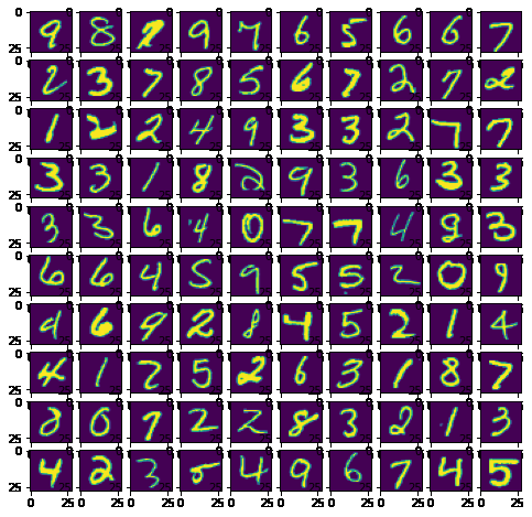
Sample images from the MNIST data
Now let’s define some hyperparameters here only so, that we can control them for the whole notebook from here only. Also, we need to reshape the data, as well as one hot encode the data to get the desired results.
Python3
num_features = 784
num_labels = 10
learning_rate = 0.05
batch_size = 128
num_steps = 5001
train_dataset = X_train.reshape(-1, 784)
train_labels = pd.get_dummies(Y_train).values
valid_dataset = X_val.reshape(-1, 784)
valid_labels = pd.get_dummies(Y_val).values
|
Computation Graph
Now, we create a computation graph. Defining a computation graph helps us to achieve the functionality of the EagerTensor that is provided by TensorFlow.
Python3
graph = tf.Graph()
with graph.as_default():
tf_train_dataset = tf1.placeholder(tf.float32,
shape=(batch_size, num_features))
tf_train_labels = tf1.placeholder(tf.float32,
shape=(batch_size, num_labels))
tf_valid_dataset = tf.constant(valid_dataset)
weights = tf.Variable(
tf.random.truncated_normal([num_features, num_labels]))
biases = tf.Variable(tf.zeros([num_labels]))
logits = tf.matmul(tf_train_dataset, weights) + biases
loss = tf.reduce_mean(tf.nn.softmax_cross_entropy_with_logits(
labels=tf_train_labels, logits=logits))
optimizer = tf1.train.GradientDescentOptimizer(
learning_rate).minimize(loss)
train_prediction = tf.nn.softmax(logits)
tf_valid_dataset = tf.cast(tf_valid_dataset, tf.float32)
valid_prediction = tf.nn.softmax(
tf.matmul(tf_valid_dataset, weights) + biases)
|
Running the Computation Graph
Since we have already built the computation graph, now it’s time to run it through a session.
Python3
def accuracy(predictions, labels):
correctly_predicted = np.sum(
np.argmax(predictions, 1) == np.argmax(labels, 1))
acc = (100.0 * correctly_predicted) / predictions.shape[0]
return acc
|
We will use the above utility function to calculate the accuracy of the model as the training goes on.
Python3
with tf1.Session(graph=graph) as session:
tf1.global_variables_initializer().run()
print("Initialized")
for step in range(num_steps):
offset = np.random.randint(0, train_labels.shape[0] - batch_size - 1)
batch_data = train_dataset[offset:(offset + batch_size), :]
batch_labels = train_labels[offset:(offset + batch_size), :]
feed_dict = {tf_train_dataset: batch_data,
tf_train_labels: batch_labels}
_, l, predictions = session.run([optimizer, loss, train_prediction],
feed_dict=feed_dict)
if (step % 500 == 0):
print("Minibatch loss at step {0}: {1}".format(step, l))
print("Minibatch accuracy: {:.1f}%".format(
accuracy(predictions, batch_labels)))
print("Validation accuracy: {:.1f}%".format(
accuracy(valid_prediction.eval(), valid_labels)))
|
Output:
Initialized
Minibatch loss at step 0: 3185.3974609375
Minibatch accuracy: 7.0%
Validation accuracy: 21.1%
Minibatch loss at step 500: 619.6030883789062
Minibatch accuracy: 86.7%
Validation accuracy: 89.0%
Minibatch loss at step 1000: 247.22283935546875
Minibatch accuracy: 93.8%
Validation accuracy: 85.7%
Minibatch loss at step 1500: 2945.78662109375
Minibatch accuracy: 78.9%
Validation accuracy: 83.6%
Minibatch loss at step 2000: 337.13922119140625
Minibatch accuracy: 94.5%
Validation accuracy: 89.0%
Minibatch loss at step 2500: 409.4652404785156
Minibatch accuracy: 89.8%
Validation accuracy: 90.6%
Minibatch loss at step 3000: 1077.618408203125
Minibatch accuracy: 84.4%
Validation accuracy: 90.3%
Minibatch loss at step 3500: 986.0247802734375
Minibatch accuracy: 80.5%
Validation accuracy: 85.9%
Minibatch loss at step 4000: 467.134521484375
Minibatch accuracy: 89.8%
Validation accuracy: 85.1%
Minibatch loss at step 4500: 1007.259033203125
Minibatch accuracy: 87.5%
Validation accuracy: 87.5%
Minibatch loss at step 5000: 342.13690185546875
Minibatch accuracy: 94.5%
Validation accuracy: 89.6%
Some important points to note:
- In every iteration, a minibatch is selected by choosing a random offset value using np.random.randint method.
- To feed the placeholders tf_train_dataset and tf_train_label, we create a feed_dict like this:
feed_dict = {tf_train_dataset : batch_data, tf_train_labels : batch_labels}
Although many of the functionalities we have implemented from scratch here are provided automatically if one uses TensorFlow. But they have been implemented from scratch to get a better intuition of the mathematical formulas which are used in the Softmax Regression Classifier.
Share your thoughts in the comments
Please Login to comment...