Skewness – Measures and Interpretation

What is Skewness?

Skewness can be defined as a statistical measure that describes the lack of symmetry or asymmetry in the probability distribution of a dataset. It quantifies the degree to which the data deviates from a perfectly symmetrical distribution, such as a normal (bell-shaped) distribution. Skewness is a valuable statistical term because it provides insight into the shape and nature of a dataset’s distribution. For example, understanding whether a dataset is positively or negatively skewed can be important in various fields, including finance, economics, and data analysis, as it can impact the interpretation of data and the choice of statistical techniques.

Tests of Skewness

There are several statistical tests and methods to assess the skewness of a dataset. These tests can help you determine whether a dataset is positively skewed, negatively skewed, or approximately symmetric. Here are some common tests and techniques used to assess skewness:

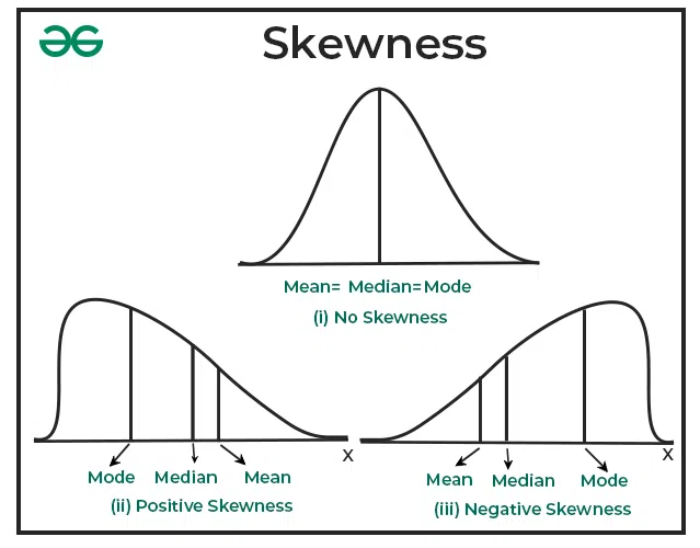
1. Visual Inspection: The simplest way to assess skewness is by creating a histogram or a density plot of the given data. If the plot is skewed to the left, it is negatively skewed, and if the plot is skewed to the right, it is positively skewed. If the plot is roughly symmetric, it has no skewness.

2. Skewness Coefficient (Pearson’s First Coefficient of Skewness): This is a numerical measure of skewness, which determines the skewness when mean and mode are not equal. It is calculated as:

Skewness as per Karl Pearson’s Measure

Skewness = Mean – Mode

Skewness of Karl Pearson’s Measure

• If mean is greater than mode, the skewness will consist positive value.
• In case of mean is smaller than mode, the skewness will be a negative value.
• In case of equality of mean and mode, the skewness will be zero.

3. Quartiles are not equidistant from each other; i.e., 

Positive and Negative Skewness

Positive skewness and negative skewness are two different ways that a dataset’s distribution can deviate from perfect symmetry (a normal distribution). They describe the direction of the skew or asymmetry in the data.

1. Positive Skewness (Right Skew)

In a positively skewed distribution, the tail on the right side (the larger values) is longer than the tail on the left side (the smaller values). This means that the majority of data points are concentrated on the left side of the distribution, and there are some extreme values on the right side. In the case of a positively skewed dataset,

Mean > Median > Mode

Examples of positively skewed data include income distribution (where most people earn a moderate income, but a few earn extremely high incomes), exam scores (where most students score in a certain range, but a few score exceptionally high), and stock market returns (where most days have modest returns, but a few days may have very high returns).

2. Negative Skewness (Left Skew)

In a negatively skewed distribution, the tail on the left side (the smaller values) is longer than the tail on the right side (the larger values). This implies that most of the data points are concentrated on the right side of the distribution, with a few extreme values on the left side. In the case of a negatively skewed dataset,

Mean < Median < Mode

Examples of negatively skewed data include test scores on an easy test (where most students score well, but a few score very low), the age at retirement (where most people retire at a certain age, but a few retire exceptionally early), and the gestational age at birth (where most babies are born full-term, but a few are born prematurely).

Measurement of Skewness

I. Karl Pearson’s Measure

Karl Pearson’s Measure of Skewness uses the mean, median, and standard deviation of the given data set to quantify the asymmetry or lack of symmetry in the distribution. It is a dimensionless number that provides valuable insights into the shape of a dataset’s distribution. This measure is valuable in various fields of statistics and data analysis, helping researchers and analysts understand the direction and degree of skewness in their datasets, which can inform subsequent modeling and analytical decisions.

Skewness as per Karl Pearson’s Measure

Skewness = Mean – Mode

Skewness of Karl Pearson’s Measure

• If mean is greater than mode, the skewness will consist positive value.
• In case mean is smaller than mode, the skewness will be a negative value.
• In case of equality of mean and mode, the skewness will be zero.

Coefficient of Skewness as per Karl Pearson’s Measure

1. With respect to Mean and Median:

2. With respect to Mean and Mode:

Here,

• S_k is Karl Pearson’s skewness coefficient.
• is the arithmetic mean or average of the data.
• M is the middle value of the data when it is arranged in ascending order.
• σ is a measure of the standard deviation of the data.

Coefficient of Karl Pearson’s Measure

• If S_k = 0, it indicates a perfectly symmetric distribution where the data is evenly balanced on both sides of the mean.
• If S_k > 0, it suggests a positively skewed distribution where the tail on the right side is longer or fatter, and the majority of data points are concentrated on the left side of the mean.
• If S_k < 0, it indicates a negatively skewed distribution where the tail on the left side is longer or fatter, and the majority of data points are concentrated on the right side of the mean.

Example of Karl Pearson’s Measure:

Calculate Pearson’s skewness coefficient for a dataset of exam scores: 85, 88, 92, 94, 96, 98, 100, 100, 100, 100.

Solution:

Step 1: Calculation of Mean

Mean = 95.3

Step 2: Calculation of Median

Since there are 10 data points, the median is the average of the 5th and 6th values when sorted in ascending order:

Median = 97

Step 3: Calculation of standard deviation.

Thus, σ=√26.81

σ = ~5.

Step 4: Calculation of mode

It is clear from the data set that 100 is the most frequently occurring value in the data. Hence, mode of given data is 100.

Step 5: Substitute the values in the formulae

A. With respect to Mean and Median

S_k = -1.02

B. With respect to Mean and Mode

S_k = -0.94

Interpretation: The skewness coefficient (Sk) is negative, indicating a slight negative skewness in the distribution of exam scores. This means that the tail of the distribution is slightly longer on the left side, and most of the scores are concentrated on the right side of the mean.

II. Bowley’s Measure

Bowley’s Skewness Coefficient, named after the British economist Arthur Lyon Bowley, is a statistical measure used to assess the skewness or asymmetry in a probability distribution. Unlike some other skewness measures that rely on moments or deviations from the mean, Bowley’s Skewness Coefficient is based on quartiles. This coefficient provides a simple and intuitive way to understand the direction and magnitude of skewness in a dataset. Bowley’s Skewness Coefficient is especially useful when dealing with data that may not follow a normal distribution or when a robust measure of skewness is required.

B = 

• Q₁ is the first quartile (25th percentile),
• Q₂ is the second quartile (50th percentile, or median), and
• Q₃ is the third quartile (75th percentile).

Coefficient of Bowley’s Measure

• If B = 0, the distribution is perfectly symmetric about the mean (no skewness).
• If B < 0, the distribution is negatively skewed (left-skewed), meaning the tail on the left side of the distribution is longer or heavier.
• If B > 0, the distribution is positively skewed (right-skewed), indicating that the tail on the right side of the distribution is longer or heavier.

Example of Bowley’s Measure:

Calculate Bowley’s Measure of Skewness for the following dataset representing the ages of a group of people in a sample: 20, 24, 28, 32, 35, 40, 42, 45, 50.

Solution:

Step 1: Calculate the median (Q₂)

Q₂= 35 (the middle value)

Step 2: Calculate the first quartile (Q₁)

To find Q₁, consider the values to the left of the median: 20, 24, 28, 32

Q₁ = 26

Step 3: Calculate the third quartile (Q₃)

To find Q₃, consider the values to the right of the median: 40, 42, 45, 50.

Q₃ = 43.5

Step 4: Substitute the above values in the formula

B = -0.02

Interpretation: Since B is negative (B < 0), the distribution is negatively skewed (left-skewed). This means that the tail of the distribution is longer on the left side, indicating that there may be outliers or high values on the right side of the data.

III. Kelly’s Measure

Kelly’s measure of skewness is a way to quantify the degree of skewness in a distribution by comparing the values of certain percentiles (typically the 10^th, 50^th, and 90^th percentiles) or deciles (10^th, 20^th, …, 90^th percentiles) of the dataset. Specifically, it involves comparing the difference between the median (50^th percentile) and the average of the 10^th and 90^th percentiles (or deciles) to assess the skewness of the data.

Skewness as per Kelly’s Measure

Coefficient of Skewness as per Kelly’s Measure

SK_L = 

Coefficient of Kelly’s Measure

• If SK_L is positive, it indicates positive skewness, meaning the distribution has a longer right tail.
• If SK_L is negative, it indicates negative skewness, meaning the distribution has a longer left tail.
• If SK_L is close to zero, it suggests that the distribution is approximately symmetric.

Example of Kelly’s Measure:

Calculate Kelly’s Coefficient of Skewness for the following data: 5, 7, 8, 9, 10, 12, 15, 16, 18, 20.

Solution:

Step 1: Find the 10^th Percentile

To find the 10^th percentile, we need to rank the data in ascending order and find the value below which 10% of the data falls. In this dataset, the 10^th percentile corresponds to the value at position 1 since 10% of 10 data points is 1. So, the 10^th percentile is 5.

P₁₀ = 5

Step 2: Find the 50^th Percentile (Median)

Since there are 10 data points, the median is the average of the 5^th and 6^th values when sorted in ascending order

P₅₀ = 11

Step 3: Find the 90^th Percentile

To find the 90^th percentile, you need to identify the value below which 90% of the data falls. In this dataset, the 90^th percentile corresponds to the value at position 9 since 90% of 10 data points is 9. So, the 90^th percentile is 18.

P₉₀ = 18

Step 4: Substitute the values in the formula.

SK_L = 0.07

Interpretation: Since the value is positive, Kelly’s Skewness Coefficient suggests that the distribution has a slight positive skewness, meaning it has a longer right tail. This indicates that there may be some data points on the right side of the distribution that are relatively larger compared to the majority of data points.

Interpretation of Skewness

Interpreting skewness involves understanding the nature of the skewness (left or right) and its magnitude. Here is how to interpret skewness:

I. Direction of Skewness:

Negative Skewness (Left Skewed): If the skewness is negative, it indicates that the distribution is skewed to the left. In a left-skewed distribution:

• The tail on the left side (the smaller values) is longer and often contains outliers.
• The majority of data points are concentrated on the right side.
• The mean is typically less than the median.

Positive Skewness (Right Skewed): A positive skewness indicates that the distribution is skewed to the right. In a right-skewed distribution:

• The tail on the right side (the larger values) is longer and may contain outliers.
• Most data points are concentrated on the left side.
• The mean is typically greater than the median.

Zero Skewness (Symmetric): A skewness value close to zero suggests a symmetric distribution where the data is evenly distributed on both sides of the mean. This means there is no skewness.

II. Magnitude of Skewness:

The magnitude of skewness provides information about the degree of skewness.

• If the skewness value is close to 0 (between -0.5 and 0.5), the distribution is approximately symmetric.
• If the skewness value is significantly negative (below -1), it suggests strong left skewness.
• If the skewness value is significantly positive (above 1), it suggests strong right skewness.

Difference between Dispersion and Skewness

Basis	Dispersion	Skewness
Focus	Focuses on the variability or spread of data points around the central tendency (mean, median).	Focuses on the shape of the distribution and the direction of the skewness (left or right).
Measurement	Common measures of dispersion include variance, standard deviation, range, and interquartile range (IQR).	Common measures of skewness include Pearson’s first coefficient of skewness, moment skewness, and graphical methods like Q-Q plots.
Relationship to Mean	Dispersion measures are not directly related to the mean, although they can affect the mean’s interpretation when it is used as a measure of central tendency.	Skewness provides information about the relationship between the mean and the median. Positive skewness implies that the mean is greater than the median, and negative skewness implies the opposite.
Interpretation	High dispersion indicates that data points are scattered or dispersed widely from the center, suggesting a wide range of values.	Positive skewness indicates a right-skewed distribution with a longer right tail, while negative skewness indicates a left-skewed distribution with a longer left tail. Zero skewness suggests a symmetric distribution.
Application	Dispersion measures are useful for understanding the variability of data and assessing how tightly or loosely data points are clustered around the central value.	Skewness is useful for understanding the shape of a distribution and identifying whether it is skewed to the left or right. It helps assess the asymmetry of the data.
Examples	Examples of dispersion include the spread of test scores in a classroom, the variability of stock prices over time, or the range of ages in a population.	Examples of skewness include income distributions (often right-skewed), response times for a website (potentially right-skewed with outliers), and exam score distributions (which can be either left-skewed or right-skewed).