Diabetes Prediction using R

In this article, we will learn how to predict whether a person has diabetes or not using the Diabetes dataset. This is a classification problem, thus we’re utilizing a Logistic regression in R Programming Language.

Here are the main steps for this project:

1. Load the dataset
2. Analyze the data
3. Exploratory data analysis(EDA)
4. Preprocessing
5. Training model
6. Evaluate model
7. Make prediction

Overview of dataset

The dataset utilized is the “diabetes.csv” dataset, which presumably contains diabetes-related information. Pregnancies, glucose levels, blood pressure, skin thickness, insulin levels, BMI (Body Mass Index), diabetes pedigree function, and age are among the factors considered. The result variable, which most likely represents the presence or absence of diabetes, is labeled “Outcome.”

1. Pregnancies: Number of times pregnant
2. Glucose: two hours following an oral glucose tolerance test, plasma glucose concentration
3. BloodPressure: Diastolic blood pressure (mm Hg)
4. SkinThickness: Triceps skinfold thickness (mm)
5. Insulin: 2-Hour serum insulin (mu U/ml)
6. BMI: Body mass index (weight in kg/(height in m)^2)
7. DiabetesPedigreeFunction: Based on family history, it is a numerical score that determines the genetic risk of diabetes. It considers the prevalence of diabetes among relatives to assess an individual’s likelihood of developing the condition. A higher DPF score indicates a greater genetic predisposition to diabetes.
8. Age: Age (years)
9. Outcome: Class variable (0 or 1)

DataSet Link: Diabetes Dataset

Load Dataset and required libraries

The code includes three R libraries for data manipulation, splitting, and modeling: “readr” for reading data, “caTools” for data splitting, and “e1071” for machine learning techniques. These libraries are widely used in data analysis and predictive modeling applications. “readr” rapidly reads data files, “caTools” provides utilities for partitioning data into training and testing sets, and “e1071” implements different machine learning algorithms, including Logistic regression. Together, these tools form a solid foundation for data preprocessing, model construction, and evaluation in R programming.

R

library(readr)
library(caTools)
library(caret)
library(e1071)

data <- read.csv("diabetes.csv")
head(data)

Output:

  Pregnancies Glucose BloodPressure SkinThickness Insulin  BMI DiabetesPedigreeFunction Age Outcome
1           6     148            72            35       0 33.6                    0.627  50       1
2           1      85            66            29       0 26.6                    0.351  31       0
3           8     183            64             0       0 23.3                    0.672  32       1
4           1      89            66            23      94 28.1                    0.167  21       0
5           0     137            40            35     168 43.1                    2.288  33       1
6           5     116            74             0       0 25.6                    0.201  30       0

The head command will print the top 6 rows of data. After running head(data) command, the table will be printed on console.

This dataset contains eight features, each of which determines a result of 0 or 1. A score of 0 means the patient does not have diabetes, whereas a score of 1 means they do.

Analyze the data

To view the dataset’s statistics, including the mean, median, lowest value, greatest value, etc., we will now use the summary command. Next, we’ll look for the missing value and drop it if it exists.

R

# Check data summary
summary(data)

# Check for missing values
colSums(is.na(data))

Output:

  Pregnancies        Glucose      BloodPressure    SkinThickness      Insulin           BMI       
 Min.   : 0.000   Min.   :  0.0   Min.   :  0.00   Min.   : 0.00   Min.   :  0.0   Min.   : 0.00  
 1st Qu.: 1.000   1st Qu.: 99.0   1st Qu.: 62.00   1st Qu.: 0.00   1st Qu.:  0.0   1st Qu.:27.30  
 Median : 3.000   Median :117.0   Median : 72.00   Median :23.00   Median : 30.5   Median :32.00  
 Mean   : 3.845   Mean   :120.9   Mean   : 69.11   Mean   :20.54   Mean   : 79.8   Mean   :31.99  
 3rd Qu.: 6.000   3rd Qu.:140.2   3rd Qu.: 80.00   3rd Qu.:32.00   3rd Qu.:127.2   3rd Qu.:36.60  
 Max.   :17.000   Max.   :199.0   Max.   :122.00   Max.   :99.00   Max.   :846.0   Max.   :67.10  
 DiabetesPedigreeFunction      Age           Outcome     
 Min.   :0.0780           Min.   :21.00   Min.   :0.000  
 1st Qu.:0.2437           1st Qu.:24.00   1st Qu.:0.000  
 Median :0.3725           Median :29.00   Median :0.000  
 Mean   :0.4719           Mean   :33.24   Mean   :0.349  
 3rd Qu.:0.6262           3rd Qu.:41.00   3rd Qu.:1.000  
 Max.   :2.4200           Max.   :81.00   Max.   :1.000  

             Pregnancies                  Glucose            BloodPressure            SkinThickness 
                       0                        0                        0                        0 
                 Insulin                      BMI DiabetesPedigreeFunction                      Age 
                       0                        0                        0                        0 
                 Outcome 
                       0 

It’s great that after reviewing our dataset, we didn’t find any null values. Even better, not a single attribute is categorical—all of them are numerical.

Moving on, let’s use exploratory data analysis (EDA) to find connections between the attributes.

Data Visualization

Now we will create some visualization for this dataset to get some informations.

Correlation Heatmap

R

# import libraries
library(ggplot2)
library(reshape2)

correlation_matrix <- cor(data)

# Convert correlation matrix to long format
correlation_melted <- melt(correlation_matrix)

# Plot heatmap
ggplot(correlation_melted, aes(Var1, Var2, fill=value)) +
  geom_tile(color="white") +
  scale_fill_gradient2(low="blue", high="red", mid="white", midpoint=0, 
                       limit=c(-1,1), space="Lab", name="Correlation") +
  theme_minimal() +
  theme(axis.text.x = element_text(angle = 45, hjust = 1)) +
  labs(title="Correlation Heatmap", x="Features", y="Features")

Output:

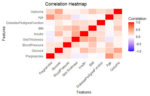
Predicting Diabetes Risk in R

Distribution of diabetes outcome

R

outcome_counts <- table(data$Outcome)
outcome_df <- data.frame(Outcome = names(outcome_counts), 
                         Count = as.numeric(outcome_counts))

# Create bar plot
ggplot(outcome_df, aes(x=Outcome, y=Count)) +
  geom_bar(stat="identity", fill="pink") +
  labs(title="Distribution of Diabetes Outcomes", x="Outcome", y="Count") +
  theme_minimal() +
  theme(axis.text.x = element_text(size=12),
        axis.text.y = element_text(size=12),
        axis.title = element_text(size=12),
        plot.title = element_text(size=16, face="bold"))

Output:

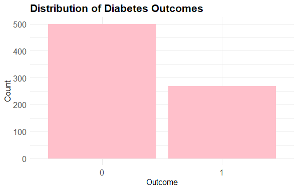
Predicting Diabetes Risk in R

Histograms with Outcome Split

R

library(ggplot2)

# Select relevant columns
diabetes_subset <- data[, c("Pregnancies", "Glucose", "BloodPressure", 
                                "BMI", "Age", "Outcome")]

# Histograms
ggplot(diabetes_subset, aes(x = Pregnancies, fill = factor(Outcome))) +
  geom_histogram(position = "identity", bins = 30, alpha = 0.7) +
  labs(title = "Distribution of Pregnancies by Outcome") +
  facet_wrap(~Outcome, scales = "free_y") +
  theme_minimal()

Output:

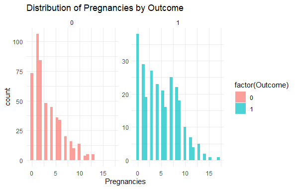
Predicting Diabetes Risk in R

Here we Compare the distribution of numerical features for positive and negative outcomes.

Boxplot for BMI by Outcome

R

library(ggplot2)

# Boxplot
ggplot(data, aes(x = factor(Outcome), y = BMI, fill = factor(Outcome))) +
  geom_boxplot() +
  labs(title = "BMI Distribution by Outcome") +
  theme_minimal()

Output:

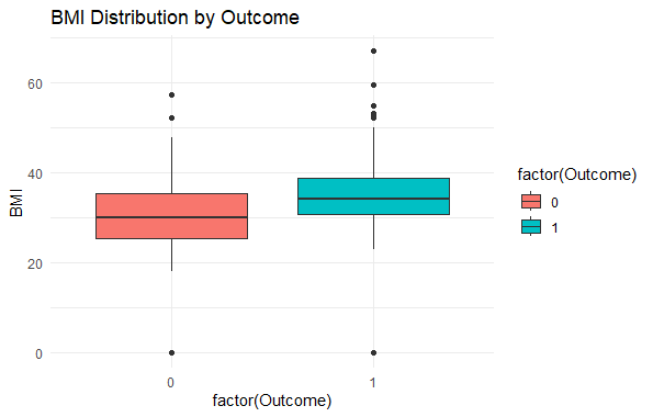
Predicting Diabetes Risk in R

Visualize the distribution of BMI for each outcome.

Data Preprocessing

1. Split data into X and y.
2. Scale features(X).
3. Bind scaled X with y
4. Split scaled data into X and y
5. Initialize the random number generator with 123 as seed value.
6. Divide the X and y into two parts: 70% for training and 30% for testing.

R

# Split data into X and y
X <- data[, 1:8]
y <- data[, 9]

# Scale only the features (X)
scaled_X <- as.data.frame(scale(X))

# Bind scaled X with y
scaled_data <- cbind(scaled_X, y)


# Split scaled data into X and y
X <- scaled_data[, 1:8]
y <- scaled_data[, 9]

# Split X and y into training and testing sets
set.seed(123)
sample <- sample.split(y, SplitRatio = 0.7)
X_train <- X[sample == TRUE, ]
y_train <- y[sample == TRUE]
X_test <- X[sample == FALSE, ]
y_test <- y[sample == FALSE]

Separate data into X and Y: This code divides the dataset into two pieces, X (features) and Y (target variable). X comprises the dataset’s first eight columns, which are referred to as features. x contains the dataset’s ninth column, which represents the goal variable (Outcome).

• Scale only the features (X): The features (X) are scaled so that the mean is 0 and the standard deviation is 1. This standardization ensures that all features are of the same scale, preventing any one component from dominating the model due to its larger magnitude.
• Bind scaled X to y: This code combines the scaled features (scaled_X) with the original target variable (y) to generate a new dataset named scaled_data. This step guarantees that the scaled features are still associated with their respective target variable.
• Split X and Y into Training and Testing Sets: The dataset is divided into training and testing sets using a 70:30 split ratio. The training set (X_train, y_train) includes 70% of the data that will be utilized to train the model. The testing set (X_test, y_test) contains the remaining 30% of the data, which will be used to assess the model’s effectiveness. The set.seed(123) function ensures reproducibility by specifying a random seed for the sampling operation.

Model Training and Evaluate

We are using Logistic regression for classification task in this project. Use below command to train the model.

R

log_model <- glm(y_train ~ ., data = X_train, family = binomial)
# Make predictions
predictions <- predict(log_model, newdata = X_test, type = "response")

# Convert predicted outcome to factor with levels matching actual outcome
predictions <- factor(ifelse(predictions > 0.5, 1, 0), 
                      levels = levels(as.factor(y_test)))

# Generate confusion matrix
confusionMatrix(predictions, as.factor(y_test))

Output:

Confusion Matrix and Statistics

          Reference
Prediction   0   1
         0 127  37
         1  23  43
                                          
               Accuracy : 0.7391          
                 95% CI : (0.6773, 0.7946)
    No Information Rate : 0.6522          
    P-Value [Acc > NIR] : 0.002949        
                                          
                  Kappa : 0.4005          
                                          
 Mcnemar's Test P-Value : 0.093290        
                                          
            Sensitivity : 0.8467          
            Specificity : 0.5375          
         Pos Pred Value : 0.7744          
         Neg Pred Value : 0.6515          
             Prevalence : 0.6522          
         Detection Rate : 0.5522          
   Detection Prevalence : 0.7130          
      Balanced Accuracy : 0.6921          
                                          
       'Positive' Class : 0  

This code uses the training data (X_train and Y_train) to train a logistic regression model (log_model). The formula y_train ~. models the target variable as a function of all variables in the training data (X_train). The family = binomial argument indicates that the logistic regression model is used for binary classification, with the response variable having a binomial distribution. Based on the input feature values, the logistic regression model determines the chance that the target variable belongs to a specific class.

This code applies the trained logistic regression model (‘log_model’) to the test data (‘X_test’) to create predictions.

• The ‘type = “response”‘ input indicates that the projected probabilities for the positive class are returned.
• These probabilities are then translated into binary predictions, with positive values above 0.5 and negative values below or equal to 0.5.
• Finally, a confusion matrix is created to assess the model’s performance by comparing the predicted values to the actual test labels (y_test).
• Accuracy: The percentage of correctly classified occurrences, or the overall accuracy of the model. The accuracy in this instance is 73.91%.
• Rate of No Information (NIR): The precision attained by consistently forecasting the most common class. The NIR in this instance is 65.22%.
• P-Value [Acc > NIR]: The statistical test’s p-value, which assesses how accurate the model is in relation to the NIR. The accuracy of the model is statistically substantially better than the NIR when the p-value is less than 0.05. The accuracy of the model in this instance is statistically considerably superior than the NIR, as indicated by the p-value of 0.002949.
• Kappa: 0.4005 (moderate agreement, -1 to 1) between the actual and predicted categories
• P-Value for Mcnemar’s Test: 0.093290 (The gap between the model’s predicted and actual classifications is not statistically significant.)
• Sensitivity: 84.67% (Accurately classifying as positive the proportion of real positive cases)
• Specificity: 53.75% (Percentage of real negative cases that were appropriately labeled as negative)
• Value of Pos Pred (PPV): 77.44% (The percentage of positive cases that are really anticipated to be positive)
• Neg Pred Value (NPV): 65.15 percent (The percentage of negative cases that are actually anticipated to be negative)
• Prevalence: 65.22% (the percentage of instances that are positive in the dataset)
• Detection Rate: 55.22% (Accurate classification of positive cases, independent of class imbalance)
• Detection Prevalence: 71.30% (Percentage of all cases, independent of actual class, classed as positive)
• Balanced accuracy: 69.21% (Mean of specificity and sensitivity)

Make a prediction

R

predict_diabetes <- function(pregnancies, glucose, bloodpressure, skinthickness, 
                             insulin, bmi, diabetespedigreefunction, age) {
  input_data <- data.frame(
    Pregnancies = pregnancies,
    Glucose = glucose,
    BloodPressure = bloodpressure,
    SkinThickness = skinthickness,
    Insulin = insulin,
    BMI = bmi,
    DiabetesPedigreeFunction = diabetespedigreefunction,
    Age = age
  )
  input <- as.data.frame(input_data)
  prediction <- predict(log_model, newdata = input, type = "response")
  prediction <- factor(ifelse(prediction > 0.5, 1, 0), 
                       levels = levels(as.factor(prediction)))
  
  return(prediction)
}

new_patient <- data.frame(
  pregnancies = 6,
  glucose = 148,
  bloodpressure = 72,
  skinthickness = 35,
  insulin = 0,
  bmi = 33.6,
  diabetespedigreefunction = 0.627,
  age = 50
)

prediction <- predict_diabetes(
  new_patient$pregnancies,
  new_patient$glucose,
  new_patient$bloodpressure,
  new_patient$skinthickness,
  new_patient$insulin,
  new_patient$bmi,
  new_patient$diabetespedigreefunction,
  new_patient$age
)

if (any(prediction == 1)) {
  cat("Based on the model's prediction, there is a higher chance of diabetes.")
} else {
  cat("Based on the model's prediction, the risk of diabetes appears lower.")
}

Output:

Based on the model's prediction, there is a higher chance of diabetes.

This code defines the function predict_diabetes, which predicts whether a new patient has diabetes depending on their medical characteristics. The program accepts input variables such as pregnancy, glucose level, blood pressure, skin thickness, insulin level, BMI, diabetes pedigree function, and age. It creates a data frame from these inputs and applies the pre-trained logistic regression model (log_model) to forecast the new patient’s diabetes risk.

• If the anticipated chance exceeds 0.5, the function returns a value of 1 (showing diabetes); otherwise, it returns 0 (indicating no diabetes). The predicted value is returned as a factor.
• A new patient’s data is then produced and provided to the predict_diabetes function, which returns the prediction. If the prediction has any values of 1 (indicating diabetes), the message “Based on the model’s prediction, there is a higher chance of diabetes” is written; otherwise, the message “Based on the model’s prediction, the risk of diabetes appears lower” is displayed.
• This code is a simple example of utilizing a logistic regression model for binary classification, specifically to predict diabetes based on medical parameters. It explains how to utilize a pre-trained model to forecast fresh data and interpret the findings to gain insight into the patient’s health status.