How do you Make a Prediction with Random Forest in R?

In the field of data science, random forests have become a tool. They are known for their ability to handle types of data prevent overfitting and provide interpretability. In this article, we shall take a look at the procedure for making forecasts with forests in R Programming Language and show how you can use an existing Iris dataset to demonstrate it.

“Random Forest”, as the name suggests, is a Classification System consisting of several Decision Trees in various Subsets and taking an average to increase their prediction accuracy.” Instead of relying on one decision tree, the random forest takes the prediction from each tree and based on the majority votes of predictions, it predicts the final output.

Getting Familiar with the Basics

The working principle of forests involves building decision trees each trained on a randomly chosen subset of data and features. This diversity helps combat overfitting issues and enhances the accuracy of the model. Once we have constructed our forest predictions are made by averaging out the tree’s predictions.

1. In the Random Forest, there are a lot of decision trees. Decision Trees, which use a tree model of decisions and their possible implications, are the key building block.
2. Ensemble training means combining the forecasts of several models to improve accuracy and robustness. A variety of decision trees, each chosen based on a specific set of data, will be created in a random Forest.
3. In Random Forest, a method known as bagging (Bootstrap Aggregating) is utilized to train decision trees on portions of the training data. This approach allows for diversity, within the ensemble like having instruments in an orchestra.

How does Random Forest Prediction work?

1. Bagging: Random Forest constructs decision trees by selecting a portion of the training data with replacement. This process, known as bootstrapped sampling involves training each tree on a subset of the data.
2. Feature Randomization: Random subsets of features are considered to be broken at each node in the tree. It ensures that there is diversity in trees, and they don’t get too correlated. A hyperparameter, which you can adjust, is a number of features that must be considered in each split.
3. Decision Tree Construction: A decision tree is created using a bootstrapped data set and random selection of features at each node, for all trees in the forest. The tree shall be grown to a minimum depth, or till the nodes are devoid of at least one sample.
4. Voting (Classification) or Averaging (Regression): When it comes to classification tasks the final prediction is determined by taking the mode, which represents the class, among all the predictions made by the trees. The average prediction for each tree is taken into account when performing regression tasks.
5. Ensemble Aggregation: The overall result of all individual trees shall be the final prediction. The use of this array approach reduces overfitting and improves the model’s generalization performance.
6. Out-of-Bag (OOB) Evaluation: Each tree in the forest is trained with a subset of data, and any other unused data are used for outofbag samples. Without the need to use a special validation set, these outofthebag samples are used for an evaluation of this model’s performance.

Difference between Random forest and decision trees

Features	Decision Trees	Random Forest
Model Structure	A single tree with rules on how to branch.	An ensemble of numerous decision trees.
Learning	Greedy, split the data so that it’s immediately improved.	Selecting the data and feature subsets randomly
Performance	Prone to overfitting and having rigid decision boundaries.	Less prone to overfitting and having smoother boundaries
Application	Quick and comprehensible models, working on small data sets	Very accurate predictions, complex problems and working on large data sets

Hyperparameters in Random Forest

1. In addition, Random Forest has a few hyperparameters that can be adjusted to optimize the model performance. In the Random Forest, here are a few key hyperparameters:
2. n_estimators: In the forest, there are a lot of decision trees. Increasing the number of trees is usually a good thing for performance, but also means higher computational costs. It is important to take account of a trade off.
3. max_depth: In a forest, the deepest depth of every decision tree. You can control the depth to avoid over fitting. More complex patterns can be captured by deeper trees, but can lead to overstuffing.
4. min_samples_split: The number of samples that need to be split in an Internal Node. The creation of nodes that represent very small subsets is prevented by higher values, reducing overfitting.
5. min_samples_leaf: To be placed on the leaf node, a minimum of samples are required. It checks when there’s excessive fitting at leaf level, as with min_samples_split. The higher value will result in a smooth boundary of the decision.
6. max_features: The maximum number of features that need to be taken into consideration for each node’s split. It may help to increase the diversity of trees and avoid excessive fitting at each split by limiting the number of characteristics considered.
7. bootstrap: Whether a bootstrapped sample should be used to build trees. if set to True enables bagging, which is a basic to the Random Forest algorithm. When each tree is trained with an unknown subset of the data, it introduces diversity.
8. random_state: Seed to generate randomly generated numbers. It ensures reproducibility. Reproducibility of results is achieved by setting the seed. A random sequence of numbers will arise from the same seed.
9. oob_score: Whether sampling from out-of-bag should be used in estimating generalization accuracy. It will provide a new evaluation metric that does not require the use of an individual validation set, if Set to True.

Steps Needed to predict random forest in R

Data Loading and Preparation

To start using your data, in R and preparing it for modeling you’ll need to follow these steps. For instance you can import data from a file using functions like read.csv(). Then ensure that the data is clean by handling missing values addressing irregularities and inconsistencies. Additionally consider feature engineering to create features as needed. Finally split your data into training and testing sets.

R

data(iris)
library(randomForest)
library(mlbench)
library(caret)

# Explore the data
head(iris)
summary(iris)

Output:

  Sepal.Length Sepal.Width Petal.Length Petal.Width Species
1          5.1         3.5          1.4         0.2  setosa
2          4.9         3.0          1.4         0.2  setosa
3          4.7         3.2          1.3         0.2  setosa
4          4.6         3.1          1.5         0.2  setosa
5          5.0         3.6          1.4         0.2  setosa
6          5.4         3.9          1.7         0.4  setosa

summary(iris)

  Sepal.Length    Sepal.Width     Petal.Length    Petal.Width          Species  
 Min.   :4.300   Min.   :2.000   Min.   :1.000   Min.   :0.100   setosa    :50  
 1st Qu.:5.100   1st Qu.:2.800   1st Qu.:1.600   1st Qu.:0.300   versicolor:50  
 Median :5.800   Median :3.000   Median :4.350   Median :1.300   virginica :50  
 Mean   :5.843   Mean   :3.057   Mean   :3.758   Mean   :1.199                  
 3rd Qu.:6.400   3rd Qu.:3.300   3rd Qu.:5.100   3rd Qu.:1.800                  
 Max.   :7.900   Max.   :4.400   Max.   :6.900   Max.   :2.500 

Random Forest Model Building

To create a forest model in R utilize the randomForest() function with parameters available for customization. These parameters include specifying the number of trees (ntree) determining how many selected features are considered at each tree node (mtry) and calculating feature importance (importance).

R

# Build the random forest model
model <- randomForest(formula = Species ~ ., data = iris, ntree = 500, mtry = 3)

# Create new data for prediction
new_data <- data.frame(Sepal.Length = 5.5, Sepal.Width = 2.3, Petal.Length = 4.1,
                       Petal.Width = 1.3)

new_data

Output:

  Sepal.Length Sepal.Width Petal.Length Petal.Width
1          5.5         2.3          4.1         1.3

Making Predictions

Once training is complete, the model can be used for data prediction. You can use prediction(), with your training model and new sets of data, to do this.

R

# Predict species of the new flower
prediction <- predict(model, newdata = new_data)

# Convert predicted species to factor with the same levels as iris$Species
predicted_species <- as.factor(prediction)
levels(predicted_species) <- levels(iris$Species)

# Print the lengths of vectors
cat("Length of predicted_species:", length(predicted_species), "\n")
cat("Number of rows in iris:", nrow(iris), "\n")

Output:

Length of predicted_species: 1 

Number of rows in iris: 150 

Model Performance Evaluation

Evaluating the accuracy and generalizability of your model involves assessing its ability to detect unobservable data.

We can utilize metrics to evaluate tasks. For regression tasks we can employ Mean Squared Error (MSE) as a measure. On the hand when it comes to classification accuracy is commonly used. Additionally confusion matrices provide insights, into the performance of classes, in classification tasks.

R

# Ensure the predicted_species vector has the same length as the number of rows in iris
predicted_species <- rep(predicted_species, nrow(iris))

# Create confusion matrix using table
conf_matrix <- table(predicted_species, iris$Species)
print(conf_matrix)

Output:

predicted_species setosa versicolor virginica
       setosa          0          0         0
       versicolor     50         50        50
       virginica       0          0         0

Begin by loading the libraries, including randomForest, mlbench and caret.

• Explore the data by displaying a preview of the rows and obtaining summary statistics, for the Iris dataset.
• Build a Random Forest model with 500 trees. Select 3 features for each split.
• Make predictions by creating data with feature values and using the model to predict the species of a newly observed flower.
• After making predictions convert the predicted species into a factor that corresponds to one of the levels observed in the dataset.
• Ensure that the length of vectors aligns with the size of the dataset and print this information.
• Evaluate model performance by creating a confusion matrix to assess accuracy, across the dataset.

Make a prediction with random forest in R

R

# Load required libraries
library(randomForest)
library(ggplot2)
library(MASS)

# Load the Boston housing dataset
data(Boston)

# Split the dataset into training and testing sets
set.seed(123)
train_indices <- sample(1:nrow(Boston), 0.7 * nrow(Boston))
train_data <- Boston[train_indices, ]
test_data <- Boston[-train_indices, ]

# Train a Random Forest regression model
rf_model <- randomForest(medv ~ ., data = train_data)

# Make predictions on the test set
predictions <- predict(rf_model, test_data)

# Visualize the predicted vs actual values
ggplot(data.frame(Predicted = predictions, Actual = test_data$medv),
       aes(x = Actual, y = Predicted)) +
  geom_point() +
  geom_abline(intercept = 0, slope = 1, color = "red", linetype = "dashed") +
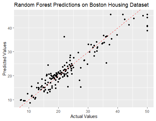
  labs(title = "Random Forest Predictions on Boston Housing Dataset",
       x = "Actual Values", y = "Predicted Values")

# Evaluate the accuracy (for regression, you might use other metrics)
accuracy <- sqrt(mean((predictions - test_data$medv)^2))
cat("Root Mean Squared Error:", accuracy, "\n")

Output:

Root Mean Squared Error: 3.38668

make a prediction with random forest in R

It will install a randomForest library, which gives you the possibility to build and analyze random forests.

• Data on Boston homes are extracted from the MASS package.
• The training and testing sets are broken down in the data set. In training, 70% of data are collected through random sampling and the remainder 30% is used to test.
• To forecast the “medv” according to any other variable, perform a regression analysis. A RMSE shall be calculated for the purpose of assessing the reliability of the regression model.
• The Root Mean Squared Error (RMSE) is used to calculate the mean magnitude of errors relative to predicted and actual values.
• Predicts the test set, using ggplot2 to show predicted versus actual values.

Advantages

1. The algorithms accuracy is generally much better, than algorithms especially when dealing with graphical data.
2. This particular model is less prone to overfitting compared to decision trees.
3. No additional processing is needed for both continuous variables.
4. It can be easily parallelized for training on datasets.
5. It also automates the identification of features reducing the need, for development.

Disadvantages

1. What goes on in a model may not be obvious to the observer, and it’s more ambiguous that any of its counterparts.
2. Training randomly produced forests can be expensive and requires a large number of memory resources.
3. Using trained forests can be quite costly. Demands a substantial amount of memory resources.
4. Properly adjusting hyperparameters is necessary. It may require some time and expert guidance.
5. When it comes to capturing the complexity of feature interactions this model may not be as efficient, as some alternatives.
6. The random nature of this algorithm could lead to behavior and slight variations in results for each run.