The DescTools package in R programming is a collection of functions that are used in various scenarios where data description, summary, and exploration are needed. It is a widely used package that was designed to help data scientists, researchers, and data analyst to understand their data and identify their findings.
The DescTools package comes with a wide range of functions that can be used in the program to understand the data better with the help of visualization. It is basically used for generating descriptive statistics, histograms, boxplots, scatterplots, and density plots. It also provides functions for calculating measures of central tendency, dispersion, correlation, and regression analysis.
Installation of DescTools
To use the DescTools package in R, you first need to install it using the following command:
R
install.packages("DescTools")
|
Now to load it into your R session use the library() function :
Now we can successfully use DescTools in your R session for generating descriptive statistics, visualizations, etc.
Functions in DescTools Package in R
The Desctools package in R programming provides a number of functions that are used to perform statistics operations. A few of them are listed below:
| |
Method |
Description |
| 1) |
SD() |
Computes the Standard Deviation |
| 2) |
range() |
Computes the range of the data |
| 3) |
mean() |
Computes the arithmetic mean |
| 4) |
median() |
Computes the middle value |
| 5) |
mode() |
Computes the most frequent values |
| 6) |
var() |
Computes variance |
| 7) |
PlotMarDens() |
Draws a Scatterplot with Marginal Density |
| 8) |
cor() |
Computes covariance or correlation |
| 9) |
AxisBreak() |
Places a break mark on the axis of an existing plot |
| 10) |
BoxCox() |
Transforms the input variable using Box-Cox transformation |
| 11) |
CartToPol |
Transforms cartesian coordinates to polar coordinates |
| 12) |
FindCorr |
Determines highly correlated variables |
| 13) |
BarText() |
Add labels on a Barplot |
| 14) |
AscToChar() |
Converts ASCII codes to Characters |
| 15) |
BinomCl() |
Computes Confidence Intervals for Binomial Proportions |
| 16) |
BinomDiffCl |
Computes confidence interval for a difference of binomials |
| 17) |
CoefVar() |
Computes coefficient of variation |
| 18) |
Cstat() |
Computes C statistic which is equivalent to the area under ROC curve |
| 19) |
moveAvg() |
Computes a simple moving average |
| 20) |
Outlier() |
Returns outliers following Tukey’s boxplot and Hampel’s median/mad definition |
| 21) |
OddsRatio() |
Computes odds ratio and confidence intervals |
| 22) |
Sample() |
Compute random samples and permutations |
| 23) |
AUC() |
Computes Area Under the Curve with a naive algorithm |
| 24) |
ZTest() |
Computes test hypothesis for a known population Standard Deviation |
| 25) |
power.chisq.test() |
Computes power calculations for ChiSquared Tests |
| 26) |
lines.lm() |
Adds a linear regression line to an existing plot |
| 27) |
StrLeft(), StrRight() |
Returns the left or right part of the string |
| 28) |
StrRev() |
Reverses a string |
| 29) |
Sort() |
Sorts a vector, matrix, table, or a dataframe |
| 30) |
TMod() |
Creates a comparison table for Linear Models |
Descriptive Statistics using DescTools Package in R
Descriptive statistics are used to summarize and describe the basic features of a dataset. The DescTools package provides functions for calculating common descriptive statistics such as mean, median, mode, standard deviation, and variance.
Let us see a few examples of the same:
Example 1: To generate descriptive statistics for a numeric variable
Syntax :
Desc(x, ..., main = NULL, plotit = NULL, wrd = NULL)
Parameters:
- x: The object to be described.
- main: A character vector, containing the main title(s). If this is left to NULL, the title will be composed as variable name (class(es)).
- plotit: It is a boolean which if true a plot is created.
- wrd: The pointer to a running MS Word instance which is default NULL, which will report all results to the console.
R
data <- c(1, 2, 3, 4, 5)
Desc(data)
|
Output :
data (numeric)

  length       n    NAs  unique    0s  mean  meanCI'
       5       5      0     = n     0  3.00    1.04
          100.0%   0.0%          0.0%          4.96

     .05     .10    .25  median   .75   .90     .95
    1.20    1.40   2.00    3.00  4.00  4.60    4.80

   range      sd  vcoef     mad   IQR  skew    kurt
    4.00    1.58   0.53    1.48  2.00  0.00   -1.91


   value  freq   perc  cumfreq  cumperc
1      1     1  20.0%        1    20.0%
2      2     1  20.0%        2    40.0%
3      3     1  20.0%        3    60.0%
4      4     1  20.0%        4    80.0%
5      5     1  20.0%        5   100.0%

' 95%-CI (classic)
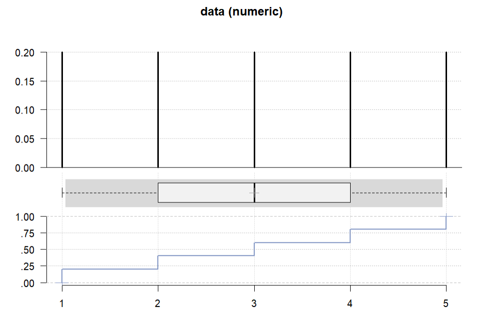
Graph for descriptive statistics for a numeric variable
Example 2: To calculate the standard deviation of a numeric variable
Syntax :
SD(x, weights = NULL, na.rm = FALSE, ...)
Parameters:
- x: A numeric vector or an R object which is coercible to one by as.double(x).
- weights: A numerical vector of weights the same length as x giving the weights to use for elements of x.
- na.rm: It is logical if true will return missing values.
R
data <- c(10, 12, 15, 18, 20, 22, 25, 27, 30)
SD(data)
|
Output :
6.80889940527183
Example 3: To calculate mean, median, mode, range, and variance
Let us first see the syntax of various descriptive statistics
i) Mean
Syntax: mean(x, trim = 0, na.rm = FALSE)
Parameter:
- x: numeric vector or data frame.
- trim: the fraction (0 to 0.5) of values to be trimmed from both ends of the data.
- na.rm: a logical value indicating whether missing values should be removed.
ii) Median
Syntax: median(x, na.rm = FALSE)
Parameter:
- x: numeric vector or data frame.
- na.rm: a logical value indicating whether missing values should be removed.
iii) Mode
Syntax: Mode(x)
Parameter:
- x: numeric vector or data frame.
iv) Range
Syntax: range(x, na.rm = FALSE)
Parameter:
- x: numeric vector or data frame.
- na.rm: a logical value indicating whether missing values should be removed.
v) Variance
Syntax: var(x, na.rm = FALSE)
Parameter:
- x: numeric vector or data frame.
- na.rm: a logical value indicating whether missing values should be removed.
R
x <- c(2, 3, 4, 5, 6, 7, 8, 9, 10)
mean(x)
median(x)
Mode <- function(x) {
ux <- unique(x)
ux[which.max(tabulate(match(x, ux)))]
}
Mode(x)
range(x)
var(x)
|
Output :
6
6
2
210
7.5
Exploratory data analysis using DescTools Package in R
Exploratory data analysis (EDA) is an approach to analyzing data to summarize their main characteristics, often with visual methods. The DescTools package provides functions for generating histograms, boxplots, and other visualizations to explore data.
Example 1: To generate a scatterplot with marginal densities with PlotMarDens() function:
Syntax :
PlotMarDens(x, y, grp = 1, xlim = NULL, ylim = NULL,
            col = rainbow(nlevels(factor(grp))),
            mardens = c("all","x","y"), pch = 1, pch.cex = 1,
            main = "", args.legend = NULL,
            args.dens = NULL, ...)
Parameters:
- x: numeric vector of x values.
- y: numeric vector of y values (of same length as x).
- grp: grouping variable(s), typically factor(s), all of the same length as x.
- xlim: the x limits of the plot.
- ylim: the y limits of the plot.
- col: the colors for lines and points. Uses rainbow() colors by default.
R
x <- rnorm(100)
y <- rnorm(100)
PlotMarDens( y, x, grp=1
, xlab="delivery_min", ylab="temperature", col=SetAlpha("brown", 0.4)
, pch=15, lwd=3
, panel.first= grid(), args.legend=NA
, main="GeekforGeeks"
)
|
Output:
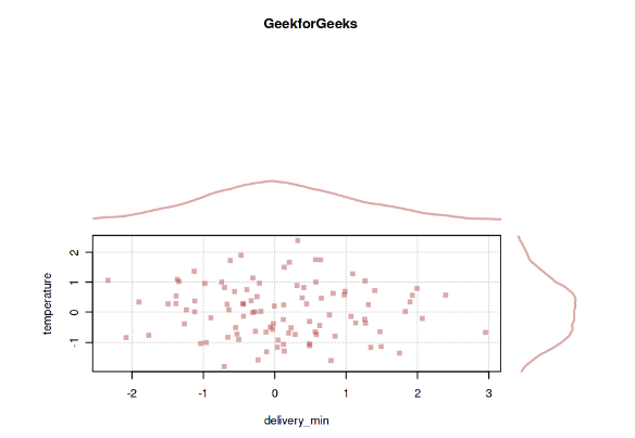
Scatterplot using PlotMarDens() function
Correlation analysis using DescTools in R
Correlation analysis is a statistical technique that measures the strength of the relationship between two variables. The DescTools package provides functions for calculating correlation coefficients and generating scatterplots to visualize relationships between variables.
Example 1: Correlation Matrix
Syntax: cor(x, use = "everything", method = c("pearson", "kendall", "spearman"))
Parameter:
- x: numeric vector or data frame.
- use: determines how to handle missing values.
- method: the method used to calculate the correlation.
Output :
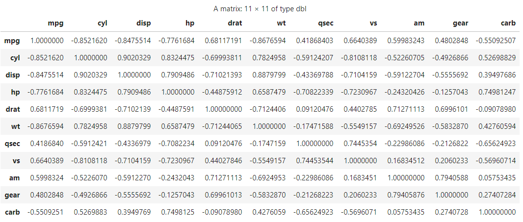
The output of Correlation Matrix
Share your thoughts in the comments
Please Login to comment...