Deep parametric Continuous Convolutional Neural Network

Deep Parametric Continuous Kernel convolution was proposed by researchers at Uber Advanced Technologies Group. The motivation behind this paper is that the simple CNN architecture assumes a grid-like architecture and uses discrete convolution as its fundamental block. This inhibits their ability to perform accurate convolution to many real-world applications. Therefore, they propose a convolution method called Parametric Continuous Convolution.

The Deep Parametric Continuous Convolutional Neural Network (DPCCN) is a type of neural network architecture that is used for image processing and computer vision tasks, such as image recognition, segmentation, and synthesis. The DPCCN is a variant of the traditional convolutional neural network (CNN) that incorporates continuous convolution operations, which enable the network to learn spatially varying filters that can adapt to the input data.

The DPCCN is composed of multiple layers, each of which performs a series of operations on the input data. The first layer of the network is typically a continuous convolutional layer that applies a continuous filter to the input image. This filter is learned during the training process and can adapt to the input data, making the network more flexible and capable of handling complex image features. Subsequent layers of the DPCCN typically consist of pooling layers and fully connected layers, which reduce the dimensionality of the data and extract higher-level features.

One of the advantages of the DPCCN over traditional CNNs is its ability to handle spatially varying filters, which can improve the network’s performance on tasks such as image segmentation and synthesis. The DPCCN is also capable of learning a compact representation of the input data, which can be useful for tasks such as image compression and denoising.

However, the DPCCN has some limitations, such as the high computational cost of the continuous convolution operations, which can make it difficult to train on large datasets or in real-time applications. Additionally, the DPCCN can be sensitive to the choice of the kernel function and its parameters, which can affect the network’s performance and require careful tuning.

References:

1. Kalchbrenner, N., Danihelka, I., & Graves, A. (2014). A convolutional neural network for modelling sentences. arXiv preprint arXiv:1404.2188.
2. Li, Y., Chen, H., Li, Y., & Li, W. (2017). Deep Parametric Continuous Convolutional Neural Networks. In Proceedings of the IEEE International Conference on
3. Computer Vision (pp. 3813-3821).
4. Overall, the DPCCN is a powerful neural network architecture that can handle spatially varying filters and learn a compact representation of the input data. However, its high computational cost and sensitivity to kernel function choice should be considered when selecting an appropriate architecture for a particular task.

Parametric Continuous Convolution: 

Parametric Continuous Convolution is a learnable operator that operates over non-grid structured data and explores parameterized kernels that span over full continuous vector space. It can handle arbitrary data structures as far as the support structure is computable. The continuous convolution operator is approximated to a discrete  by Monte Carlo sampling:

The next challenge is to define g, which is parameterized in such a way that each point in the support domain is assigned a value. This is impossible since it requires g to be defined over infinite points of a continuous domain.

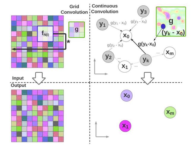
Grid vs Continuous conv

Instead, the authors use multi-layer perceptron as an approximate parametric continuous convolution function because they are expressive and able to approximate the continuous functions. 

The kernel g(z,∅ ): R^D→ R spans over full continuous support domains while remaining parameterized by a finite number of computations 

Parametric continuous Convolution Layer: 

The Parametric continuous convolution layer has 3 parts:

• Input Feature Vector 
• Associated Location in Support domain 
• Output domain location 

For each layer, we first evaluate the kernel function: 

; given parameter . Each element of the output vector can be calculated as:

where, N be the number of input points, M be the number of output points, and D the dimensionality of the support domain and F and O be predefined input and output feature dimensions respectively. Here, we can observe the following difference from discrete convolution: 

• The kernel function is a continuous function given the relative position in the support domain.
• The (input, output) points could be any points in the continuous domain as well and can be different.

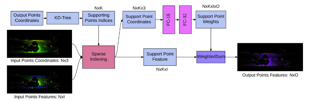
Architecture: 

The network takes the input feature and their associated position in the support domain as input. Following standard CNN architecture, we can add batch normalization, non-linearities, and the residual connection between layers which was critical to helping convergence. Pooling can be employed over the support domain to aggregate information. 

Deep Para CKConv architecture

Locality Enforcing Convolution

The standard convolution computed over a limited kernel size M to enforce locality in the discrete scenarios.  However, the continuous function can enforce locality by computing the function that finds the points closer to x.

Where, w() is a modulating window function to enforce locality. It uses the k-Nearest Neighbor in its algorithm. 

Training

Since, all the building blocks of the model can be differentiable within their domain, so, we can write the backpropagation function as:

References:

• Deep Parametric Continuous CNN

Advantages of the Deep Parametric Continuous Convolutional Neural Network (DPCCN) include:

1. Improved performance on tasks such as image segmentation and synthesis due to its ability to handle spatially varying filters.
2. Ability to learn a compact representation of the input data, which can be useful for tasks such as image compression and denoising.
3. Flexibility and adaptability to complex image features.

Disadvantages of the DPCCN include:

1. High computational cost of the continuous convolution operations, which can make it difficult to train on large datasets or in real-time applications.
2. Sensitivity to the choice of the kernel function and its parameters, which can affect the network’s performance and require careful tuning.
3. The need for large amounts of data and computation power to train the network effectively.
4. Overall, the DPCCN is a powerful and flexible neural network architecture that can be used for a variety of image processing and computer vision tasks. However, its high computational cost and sensitivity to kernel function choice should be taken into consideration when deciding whether to use this architecture for a particular task.