DALEX package in R Programming Language is useful for data scientists analysts, and stakeholders as it is designed to provide tools for model-agnostic exploration, explanation, and visualization of predictive models. R is a statistical programming language widely used for data analysis because of these user-friendly packages and libraries.
DALEX Package in R
DALEX Package can be briefed as a model Agnostic Language for Exploration and Explanation. It is popularly used to enhance the interpretability of machine learning models, making it easier to understand and trust the predictions made by these models.
Key features of the DALEX Package
- Model-Agnostic Exploratory Data Analysis: We used the word model-agnostic, which means this package can work with any predictive model irrespective of its algorithm and technique.
- Exploration of Model Behavior: This package helps understand the model’s behavior, analyzing the variable’s importance and how the variable affects the prediction.
- Explanations for Model Predictions: This package explains an individual prediction explaining why that particular prediction was made. This helps in improving the trust in the model.
- Model Diagnostics: This package also helps in analyzing the performance of the model by observing its behavior over different subsets and how it handles certain points.
- Visualization: DALEX provides a range of visualization functions to create informative plots.
- Comparison of Models: DALEX provides comparison between different packages making it easier to choose which model is better.
- Integration with Other R Packages: This package works well with other packages like “caret”, “randomForest” or “ggplot2”.
Primary Uses of the DALEX Package
- Interpretability: This package makes it easier to understand how the model works and reaches the prediction. Therefore, it is easy to interpret and user-friendly.
- Visualization: DALEX helps in building informative plots for a better understanding of model behavior and variable importance.
- Diagnostic Analysis: It also helps in the analysis of the performance of the model.
- Model Comparison: DALEX helps in the comparison of different models so that users can select the model that is better for them.
DALEX Package using iris dataset
Step-1 Load Necessary Packages
First we need to install the necessary packages for analysis of iris dataset.
R
install.packages(c("DALEX", "ggplot2"))
library(DALEX)
library(ggplot2)
|
Step 2: Load and Explore the iris Dataset
In this example, we will use in-built dataset in R. It is a very famous dataset called “iris” which have information about different flowers.
R
data(iris)
head(iris)
selected_features <- c("Sepal.Length", "Sepal.Width", "Petal.Length", "Petal.Width",
"Species")
iris_data <- iris[, selected_features]
head(iris_data)
|
Output:
Sepal.Length Sepal.Width Petal.Length Petal.Width Species
1          5.1         3.5          1.4         0.2  setosa
2          4.9         3.0          1.4         0.2  setosa
3          4.7         3.2          1.3         0.2  setosa
4          4.6         3.1          1.5         0.2  setosa
5          5.0         3.6          1.4         0.2  setosa
6          5.4         3.9          1.7         0.4  setosa
Step 3: Split the Data into Training and Testing Sets
Here, we are splitting data into training and testing sets. sample() function is used to put 70% data into training sets.
R
set.seed(123)
split_index <- sample(1:nrow(iris_data), 0.7 * nrow(iris_data))
train_data <- iris_data[split_index, ]
test_data <- iris_data[-split_index, ]
|
Step 4: Perform Modeling (Linear Regression)
Here we are modeling our data using Linear regression model. lm() function is used to fit linear regression model. Here the model will predict Sepal length using all the other variables present in it.
R
model <- lm(Sepal.Length ~ ., data = train_data)
|
Step 5: Create a DALEX Explainer
An explainer is created in DALEX model from explain() function which takes actual data, test data and response values as argument.
R
explainer <- explain(model,
data = as.data.frame(test_data[, -1]),
y = as.numeric(test_data$Sepal.Length),
label = "Linear Regression Model")
|
Output:
Preparation of a new explainer is initiated
  -> model label       :  Linear Regression Model
  -> data              :  45  rows  4  cols
  -> target variable   :  45  values
  -> predict function  :  yhat.lm  will be used (  default  )
  -> predicted values  :  No value for predict function target column. (  default  )
  -> model_info        :  package stats , ver. 4.3.1 , task regression (  default  )
  -> predicted values  :  numerical, min =  4.666851 , mean =  5.833996 , max =  7.041814
  -> residual function :  difference between y and yhat (  default  )
  -> residuals         :  numerical, min =  -0.6926251 , mean =  0.008225818 , max =  0.5184108
  A new explainer has been created!
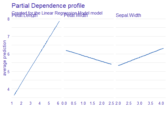
Step 6: Generate Plots for EDA using DALEX
- Variable Profiles: Visualization of the effect of each variable on predictions.
- Variable Importance: Importance scores of each variable in the model.
- Model Performance: Visualization of the model’s performance on the test data.
R
plot(model_profile(explainer))
|
Output:
DALEX Package in R
Plot Variable Importance
R
plot(variable_importance(explainer))
|
Output:

DALEX Package in R
Plot Model Performance
R
plot(model_performance(explainer))
|
Output:

DALEX Package in R
Step 7: Prediction and Comparison
New data is created for predictions, and the predict function is used with the explainer to obtain predicted values. The results are then displayed for comparison.
R
new_data <- test_data[sample(nrow(test_data), 5), selected_features[-1]]
predictions <- predict(explainer, new_data)
cbind(new_data, Predicted_Sepal_Length = predictions)
|
Output:
Sepal.Width Petal.Length Petal.Width    Species Predicted_Sepal_Length
101         3.3          6.0         2.5  virginica               6.992625
140         3.1          5.4         2.1  virginica               6.510664
116         3.2          5.3         2.3  virginica               6.404969
65          2.9          3.6         1.3 versicolor               5.426833
83          2.7          3.9         1.2 versicolor               5.625434
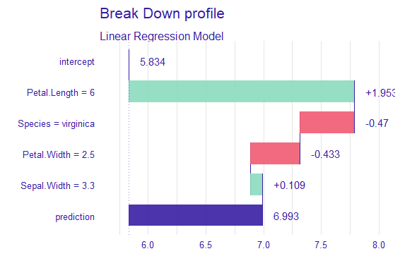
Step 8: Additional Functionalities
Shapley Additive explanations (SHAP) helps us in understanding the contribution of features in all possible combinations. These values determine the Breakdown Plot in DALEX package.
R
shap_values <- predict_parts(explainer, new_data)
plot(shap_values, type = "bar", bar_width = 0.7)
|
Output:
DALEX Package in R
Breakdown Profile are horizontal bars showing the contribution of each variable. Positive plots show higher predictions where as negative bars push the predictions lower.
Price Analysis using DALEX Package
Step 1: Load Necessary Packages:
- randomForest: It is a package used to fit a random forest model used for constructing multiple decision trees during training of the model.
- pROC: This is used for analyzing and visualizing the performance of binary classifiers. It helps evaluate metrics such as ROC, AUC, sensitivity or specificity, etc.
- PRROC: This package focuses on precision-recall curves and related metrics, particularly for binary classification problems.
- ggplot2: ggplot2 library stands for the grammar of graphics, popular because of its declarative syntax used to visualize and plot our data into graphs for better understanding.
- rpart: This package serves the main function of creating decision tree models. It is designed for building decision trees.
- gbm: This package builds gradient boosting models, specifically Gradient Boosting Machines (GBM).
- reshape2: This package is used for reshaping and transforming data frames. It provides functions like melt() which converts data from wide format to long format by melting it, used when we have to gather columns and rows.
R
install.packages(c("DALEX", "randomForest", "pROC", "PRROC"))
library(DALEX)
library(randomForest)
library(pROC)
library(PRROC)
|
After installing the necessary packages we will create the fictional dataset.
Step 2: Generate fictional data
In this example, we will create a fictional dataset based on the number of rooms, square footage, and proximity to the city center to predict the price of the house based on all these attributes mentioned.
R
set.seed(123)
n_obs <- 1000
rooms <- sample(2:6, n_obs, replace = TRUE)
square_footage <- rnorm(n_obs, mean = 1500, sd = 300)
proximity_to_center <- rnorm(n_obs, mean = 10, sd = 5)
prices <- 50000 + 10000 * rooms + 30 * square_footage - 500 * proximity_to_center +
rnorm(n_obs, mean = 0, sd = 50000)
housing_data <- data.frame(rooms, square_footage, proximity_to_center, prices)
head(housing_data)
|
Output:
  rooms square_footage proximity_to_center     prices
1     4       1844.534            6.201993 139380.295
2     4       1115.020           14.861848   6251.566
3     3       1676.837            4.840798 168033.784
4     3       1410.490           13.842933 147641.228
5     4       1516.134           11.506425  39428.894
6     6       1860.392           12.122803 147117.460
Step 3: Perform EDA (Exploratory Data Analysis)
We can perform Exploratory Data Analysis on this dataset to get insights about it. We will use the head() function to get the first six rows of the dataset. We can perform various plots with the help of the explained function of the DALEX package. The explain function in the DALEX package is used to create an explainer object for the model. This explainer object is then used to generate various plots for exploratory data analysis.
Here we are modeling the dataset using a linear regression model. lm() function is used for this modeling.
R
head(housing_data)
model <- lm(prices ~ rooms + square_footage + proximity_to_center, data = housing_data)
explainer <- explain(model,
data = as.data.frame(housing_data[, -4]),
y = as.numeric(housing_data$prices))
plot(model_profile(explainer))
plot(variable_importance(explainer))
plot(model_performance(explainer))
|
Output:
 rooms square_footage proximity_to_center     prices
1     4       1844.534            6.201993 139380.295
2     4       1115.020           14.861848   6251.566
3     3       1676.837            4.840798 168033.784
4     3       1410.490           13.842933 147641.228
5     4       1516.134           11.506425  39428.894
6     6       1860.392           12.122803 147117.460
preparation of a new explainer is initiated
  -> model label       :  lm  (  default  )
  -> data              :  1000  rows  3  cols
  -> target variable   :  1000  values
  -> predict function  :  yhat.lm  will be used (  default  )
  -> predicted values  :  No value for predicting function target column. (  default  )
  -> model_info        :  package stats , ver. 4.3.0 , task regression (  default  )
  -> predicted values  :  numerical, min =  85242.24 , mean =  130242.6 , max =  179817.7
  -> residual function :  difference between y and yhat (  default  )
  -> residuals         :  numerical, min =  -157733.2 , mean =  2.229695e-10 , max =  141987.6
  A new explainer has been created!
- Model label: This represents the name of the model, which is linear regression here(lm)
- Data: This gives dataset information showing 1000 rows and 3 columns here
- Target Variable: This shows the number of target variables which is 1000 here
- Predict function: This shows the function used to predict, yhat.lm is used here.
- Predicted Values: This shows the characteristics of the predicted values, here it shows it is a numerical value having a minimum value of 85242.24, a mean value of 130242.6, and a maximum value of 179817.7
- Model Information: This provides details about the package, the version, and the model type.
- Residual Function: Specifies the function used to calculate residuals.
- Residuals Statistics: Describes the characteristics of the residuals.
- A new explainer has been created based on the model, data, and settings.

DALEX Package in R
A Reverse Cumulative Distribution (RCDF) plot of model residuals provides a graphical representation of how the residuals are distributed across different quantiles.
- Here, the PDP plot shows a linear increase and decrease in respective features, it suggests a proportional relationship between the number of rooms and the average predicted prices.
- A Feature Importance Plot based on RMSE (Root Mean Squared Error) loss after permutations is a way to assess the importance of each feature in a predictive model.
Features with larger bars in the plot indicate higher importance. The room has the longest bar which means it indicates higher importance here.
Step 4: Train the model
We can train the model with multiple algorithms or techniques because DALEX supports these models, so in this example, we will train the model with multiple models.
- Decision Tree Model: When training the model using the DALEX framework, we can explore the decision boundaries created by the tree, understand feature importance, and interpret how the model arrives at specific predictions.
- Random Forest Model:By utilizing DALEX to train a Random Forest model, we can delve into the ensemble’s collective behavior. The framework allows us to analyze the impact of each tree, assess feature importance across the entire forest, and understand how the model generalizes to different subsets of the data.
R
install.packages("rpart")
install.packages("randomForest")
install.packages("gbm")
library(rpart)
library(randomForest)
library(gbm)
tree_model <- rpart(prices ~ rooms + square_footage + proximity_to_center,
data = housing_data)
explainer_tree <- explain(tree_model,
data = as.data.frame(housing_data[, -4]),
y = as.numeric(housing_data$prices))
forest_model <- randomForest(prices ~ rooms + square_footage + proximity_to_center,
data = housing_data)
explainer_forest <- explain(forest_model,
data = as.data.frame(housing_data[, -4]),
y = as.numeric(housing_data$prices))
gbm_model <- gbm(prices ~ rooms + square_footage + proximity_to_center,
data = housing_data, distribution = "gaussian", n.trees = 100,
interaction.depth = 3)
explainer_gbm <- explain(gbm_model,
data = as.data.frame(housing_data[, -4]),
y = as.numeric(housing_data$prices))
|
Output:
For the Decision Tree Model
Preparation of a new explainer is initiated
  -> model label       :  rpart  (  default  )
  -> data              :  1000  rows  3  cols
  -> target variable   :  1000  values
  -> predict function  :  yhat.rpart  will be used (  default  )
  -> predicted values  :  No value for predict function target column. (  default  )
  -> model_info        :  package rpart , ver. 4.1.23 , task regression (  default  )
  -> predicted values  :  numerical, min =  111777.4 , mean =  130242.6 , max =  181098.5
  -> residual function :  difference between y and yhat (  default  )
  -> residuals         :  numerical, min =  -174279 , mean =  -4.697604e-12 , max =  150307.6
  A new explainer has been created!
For Random Forest Model
Preparation of a new explainer is initiated
  -> model label       :  randomForest  (  default  )
  -> data              :  1000  rows  3  cols
  -> target variable   :  1000  values
  -> predict function  :  yhat.randomForest  will be used (  default  )
  -> predicted values  :  No value for predict function target column. (  default  )
  -> model_info        :  package randomForest , ver. 4.7.1.1 , task regression (  default  )
  -> predicted values  :  numerical, min =  58784.43 , mean =  130272.5 , max =  187559.8
  -> residual function :  difference between y and yhat (  default  )
  -> residuals         :  numerical, min =  -124211.2 , mean =  -29.92675 , max =  110599.9
  A new explainer has been created!
For Gradient Boosting Model
Preparation of a new explainer is initiated
  -> model label       :  gbm  (  default  )
  -> data              :  1000  rows  3  cols
  -> target variable   :  1000  values
  -> predict function  :  yhat.gbm  will be used (  default  )
  -> predicted values  :  No value for predict function target column. (  default  )
  -> model_info        :  package gbm , ver. 2.1.8.1 , task regression (  default  )
  -> predicted values  :  numerical, min =  79831.99 , mean =  130586.4 , max =  187989.1
  -> residual function :  difference between y and yhat (  default  )
  -> residuals         :  numerical, min =  -149385.9 , mean =  -343.7869 , max =  132875.4
  A new explainer has been created!
Step 5: Predicting Values
Now, we will predict values for house prices based on the rooms, proximity to the center, and square footage of the house. These values help in predicting the prices of the house based on different models used for training.
R
new_data <- data.frame(rooms = c(3, 4, 5),
square_footage = c(1600, 1800, 2000),
proximity_to_center = c(8, 12, 10))
predictions_linear <- predict(explainer, new_data)
predictions_tree <- predict(explainer_tree, new_data)
predictions_forest <- predict(explainer_forest, new_data)
predictions_gbm <- predict(explainer_gbm, new_data)
cbind(new_data, Linear_Regression = predictions_linear,
Decision_Tree = predictions_tree,
Random_Forest = predictions_forest,
Gradient_Boosting = predictions_gbm)
|
Output:
rooms square_footage proximity_to_center Linear_Regression Decision_Tree
1     3           1600                   8          110133.2      111777.4
2     4           1800                  12          146651.3      137586.1
3     5           2000                  10          136265.4      140657.1
  Random_Forest Gradient_Boosting
1      110068.8          119179.9
2      143026.2          138627.7
3      135331.1          150264.1
Here we are predicting House Prices based on different models for three different scenarios
1. Scenario 1:
- Number of Rooms (rooms): 3
- Square Footage (square_footage): 1600
- Proximity to Center (proximity_to_center): 8
- Linear Regression Prediction (Linear_Regression): $110,133.2
- Decision Tree Prediction (Decision_Tree): $111,777.4
- Random Forest Prediction (Random_Forest): $110,068.8
- Gradient Boosting Prediction (Gradient_Boosting): $119,179.9
2. Scenario 2:
- Number of Rooms (rooms): 4
- Square Footage (square_footage): 1800
- Proximity to Center (proximity_to_center): 12
- Linear Regression Prediction (Linear_Regression): $146,651.3
- Decision Tree Prediction (Decision_Tree): $137,586.1
- Random Forest Prediction (Random_Forest): $143,026.2
- Gradient Boosting Prediction (Gradient_Boosting): $138,627.7
3. Scenario 3:
- Number of Rooms (rooms): 5
- Square Footage (square_footage): 2000
- Proximity to Center (proximity_to_center): 10
- Linear Regression Prediction (Linear_Regression): $136,265.4
- Decision Tree Prediction (Decision_Tree): $140,657.1
- Random Forest Prediction (Random_Forest): $135,331.1
- Gradient Boosting Prediction (Gradient_Boosting): $150,264.1
We can also visualize these values by plotting them on graphs for which we will use the ggplot2 package in R. This plot is to compare the predicted prices by different models.
Density Plot – Distribution of Predicted Prices with Different Colors
A density plot is a graphical representation of the distribution of a continuous variable. It explains the concentration on the graph
R
ggplot(predicted_prices_melted, aes(x = Predicted_Price, fill = Model)) +
geom_density(alpha = 0.7) +
labs(title = "Distribution of Predicted Prices by Different Models",
x = "Predicted Price", y = "Density") +
theme_minimal() +
scale_fill_manual(values = c(
"Linear_Regression" = "darkgreen",
"Decision_Tree" = "blue",
"Random_Forest" = "purple",
"Gradient_Boosting" = "orange"
)) +
theme(
plot.title = element_text(color = "darkgreen", size = 16, face = "bold"),
axis.title = element_text(color = "darkgreen", size = 12, face = "bold"),
legend.position = "bottom",
legend.title = element_blank(),
legend.text = element_text(color = "darkgreen", size = 10)
)
|
Output:

DALEX Package in R
Higher Peaks suggest areas where the concentration is higher, in this graph the peak for the decision tree is highest. It also explains the skewness, a longer tail on one side suggests skewness in that particular direction.
Step 6 Model Analysis
Residual Analysis is a way of evaluating the performance of a regression model. Residuals are the differences between the observed values and the values predicted by the model.
R
model_residuals <- residuals(explainer)
mean_abs_residual <- mean(abs(model_residuals))
mean_squared_residual <- mean(model_residuals^2)
root_mean_squared_residual <- sqrt(mean_squared_residual)
cat("Mean Absolute Residual:", mean_abs_residual, "\n")
cat("Mean Squared Residual:", mean_squared_residual, "\n")
cat("Root Mean Squared Residual:", root_mean_squared_residual, "\n")
|
Output:
Mean Absolute Residual: 38531.25
Mean Squared Residual: 2387179083
Root Mean Squared Residual: 48858.77
Mean Absolute Residual: The average absolute difference between the observed and predicted prices is approximately $38531.25
Mean Squared Residual: The average of the squared differences between the observed and predicted prices is approximately $2387179083. This is sensitive to large errors.
Root Mean Squared Residual: The square root of the mean squared residual is approximately $48858.77. This represents the average magnitude of errors in the response variable.
Conclusion
We learned how to use different functions of the DALEX package in estimating the house prices based on variables such as rooms, square footage, etc. We also understood DALEX package with the help of Iris dataset in R . We also visualized different plots for a better understanding of the dataset.
Share your thoughts in the comments
Please Login to comment...