Car package in R

In R, there are several packages available that provide functions and tools to perform various tasks related to data analysis and visualization. The “car” package is one of the packages that provide functions and tools for regression analysis. In this article, we will provide a comprehensive and in-depth guide to the “car” package in R, including how to install and load the package, how to use the functions it provides, and how to visualize the results.

Installing the “car” Package

Before we can start using the functions provided by the “car” package, we need to install it. Installing the “car” package can be done using the following code:

install.packages("car")

Loading the “car” Package

Once the “car” package is installed, we need to load it into the R environment. Loading the “car” package can be done using the following code:

library(car)

Example 1: Simple Linear Regression

Step 1: Data Preparation

For just demonstration purposes, we will use the “mtcars” dataset that is available in the R environment. The “mtcars” contains data on 32 different models of cars and includes information like miles per gallon (mpg), number of cylinders (cyl), horsepower (hp), weight (wt), and acceleration (qsec).

R

summary(mtcars)

Output:

     mpg             cyl             disp             hp       
 Min.   :10.40   Min.   :4.000   Min.   : 71.1   Min.   : 52.0  
 1st Qu.:15.43   1st Qu.:4.000   1st Qu.:120.8   1st Qu.: 96.5  
 Median :19.20   Median :6.000   Median :196.3   Median :123.0  
 Mean   :20.09   Mean   :6.188   Mean   :230.7   Mean   :146.7  
 3rd Qu.:22.80   3rd Qu.:8.000   3rd Qu.:326.0   3rd Qu.:180.0  
 Max.   :33.90   Max.   :8.000   Max.   :472.0   Max.   :335.0  
      drat             wt             qsec             vs        
 Min.   :2.760   Min.   :1.513   Min.   :14.50   Min.   :0.0000  
 1st Qu.:3.080   1st Qu.:2.581   1st Qu.:16.89   1st Qu.:0.0000  
 Median :3.695   Median :3.325   Median :17.71   Median :0.0000  
 Mean   :3.597   Mean   :3.217   Mean   :17.85   Mean   :0.4375  
 3rd Qu.:3.920   3rd Qu.:3.610   3rd Qu.:18.90   3rd Qu.:1.0000  
 Max.   :4.930   Max.   :5.424   Max.   :22.90   Max.   :1.0000  
       am              gear            carb      
 Min.   :0.0000   Min.   :3.000   Min.   :1.000  
 1st Qu.:0.0000   1st Qu.:3.000   1st Qu.:2.000  
 Median :0.0000   Median :4.000   Median :2.000  
 Mean   :0.4062   Mean   :3.688   Mean   :2.812  
 3rd Qu.:1.0000   3rd Qu.:4.000   3rd Qu.:4.000  
 Max.   :1.0000   Max.   :5.000   Max.   :8.000  

Step 2: Simple Linear Regression

The “car” package provides functions for performing linear regression analysis. To perform simple linear regression analysis, we can use the lm() function. For example, if we want to perform a simple linear regression analysis to predict the miles per gallon (mpg) of a car based on its weight (wt), we can use the following code:

R

model <- lm(mpg ~ wt, data = mtcars)

Step 3: Model Summary

Once we have fit a linear regression model, we can get a summary of the model using the summary() function. The summary of the model provides information such as the coefficients of the regression equation, the R-squared value, and the p-value of the regression coefficients. To get the summary of the model, we can use the following code:

R

summary(model)

Output:

Call:
lm(formula = mpg ~ wt, data = mtcars)

Residuals:
    Min      1Q  Median      3Q     Max 
-4.5432 -2.3647 -0.1252  1.4096  6.8727 

Coefficients:
            Estimate Std. Error t value Pr(>|t|)    
(Intercept)  37.2851     1.8776  19.858  < 2e-16 ***
wt           -5.3445     0.5591  -9.559 1.29e-10 ***
---
Signif. codes:  0 ‘***’ 0.001 ‘**’ 0.01 ‘*’ 0.05 ‘.’ 0.1 ‘ ’ 1

Residual standard error: 3.046 on 30 degrees of freedom
Multiple R-squared:  0.7528,    Adjusted R-squared:  0.7446 
F-statistic: 91.38 on 1 and 30 DF,  p-value: 1.294e-10

Step 4: Plotting the Regression Line

The “car” package also provides functions for visualizing the results of the regression analysis. To plot the regression line, we can use the abline() function. The abline() function takes the parameters of the regression equation as inputs and plots the regression line on a scatter plot of the data. To plot the regression line, we can use the following code:

R

plot(mtcars$wt, mtcars$mpg)
abline(model)

Output:

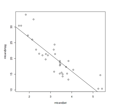
Regression line with scatter plot

Step 5: Residual Plot

The residual plot is a plot of the residuals (the differences between the observed values and the predicted values) against the fitted values. The residual plot can be used to assess the assumptions of the linear regression model, such as the assumption of homoscedasticity (constant variance of the residuals). To plot the residual plot, we can use the residplot() function provided by the “car” package. The residplot() function takes the linear regression model as an input and plots the residual

R

# Plot residuals against the fitted values
residualPlots(model)

Output:

           Test stat Pr(>|Test stat|)   
wt             3.258         0.002860 **
Tukey test     3.258         0.001122 **
---
Signif. codes:  0 ‘***’ 0.001 ‘**’ 0.01 ‘*’ 0.05 ‘.’ 0.1 ‘ ’ 1

Pearson  Residual for wt, and Fitted values

Example 2: Multiple Linear Regression

Step 1: Fit a multiple linear regression model to predict mpg based on wt and hp

R

# Load the "car" package
library(car)

# Fit a multiple linear regression model to predict mpg based on wt and hp
model <- lm(mpg ~ wt + hp, data = mtcars)

# Summary of the model
summary(model)

Output:

Call:
lm(formula = mpg ~ wt + hp, data = mtcars)

Residuals:
   Min     1Q Median     3Q    Max 
-3.941 -1.600 -0.182  1.050  5.854 

Coefficients:
            Estimate Std. Error t value Pr(>|t|)    
(Intercept) 37.22727    1.59879  23.285  < 2e-16 ***
wt          -3.87783    0.63273  -6.129 1.12e-06 ***
hp          -0.03177    0.00903  -3.519  0.00145 ** 
---
Signif. codes:  0 ‘***’ 0.001 ‘**’ 0.01 ‘*’ 0.05 ‘.’ 0.1 ‘ ’ 1

Residual standard error: 2.593 on 29 degrees of freedom
Multiple R-squared:  0.8268,    Adjusted R-squared:  0.8148 
F-statistic: 69.21 on 2 and 29 DF,  p-value: 9.109e-12

Step 2: Plot the model

R

# Plot the model
# Rsiidual vs Fitteted, Normal Q-Q, scale-location, etc
plot(model)

Output:

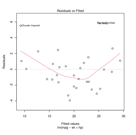
residuals  vs fitted values

Above is the scatter plot of the residuals against the fitted values. The plot is used to check for the presence of nonlinearity in the model.

Normal Q-Q plot

The Normal Q-Q plot checks for the assumption of normality by comparing the distribution of the residuals to a normal distribution. 

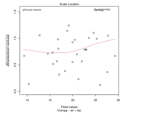
Scale-Location

The above is a plot of the square root of the absolute values of the standardized residuals against the fitted values. It is used to check for the presence of heteroscedasticity (unequal variances of the residuals). If it shows a horizontal line with equally spread points, then it suggests that the residuals have equal variance across the range of fitted values.

Residual vs Leverage

Above is the plot of the standardized residuals against the leverage of each observation. The leverage is a measure of how much an observation affects the regression line. The plot is used to identify influential observations, which are observations that have a high leverage and a large standardized residual. Influential observations can have a significant impact on the regression results and should be examined more closely.

Step 3: Plot the model

R

# Plot residuals against the fitted values
residualPlots(model)

Output:

           Test stat Pr(>|Test stat|)    
wt            3.1383        0.0039785 ** 
hp            2.4973        0.0186653 *  
Tukey test    3.7968        0.0001466 ***
---
Signif. codes:  0 ‘***’ 0.001 ‘**’ 0.01 ‘*’ 0.05 ‘.’ 0.1 ‘ ’ 1

Pearson  Residual for wt, hp, and Fitted values

Example 3: Anova and diagnostic Plots

Step 1: Perform ANOVA on the model

R

library(car)

# Fit a multiple linear regression model to predict mpg based on wt and hp
model <- lm(mpg ~ wt + hp, data = mtcars)

# Perform anova on the model
anova(model)

Output:

            A anova: 3 × 5
             Df           Sum Sq        Mean Sq        F value        Pr(>F)
           <int>        <dbl>        <dbl>        <dbl>        <dbl>
  wt        1          847.72525        847.725250    126.04109    4.488360e-12
  hp        1          83.27418        83.274183    12.38133    1.451229e-03
Residuals    29          195.04775        6.725785    NA             NA

The ANOVA function in the above example performs an analysis of variance (ANOVA) on the model that tests the significance of the overall model and the individual variables in the model.

Step 2:  Plot partial regression plots for the variables in the model

The plot function creates four plots of the partial regression plots for variables in the model which is useful for understanding the relationship between each variable and the response variable. The partial regression plot shows the relationship between the response variable and each predictor variable which has control for other predictor variables in the model. It allows you to see the unique contribution of each variable to the model and to identify any potential interactions between the variables.

R

# Plot partial regression plots for the variables in the model
par(mfrow=c(2,2))
plot(model, which=c(1,2,3,4,5))

Output:

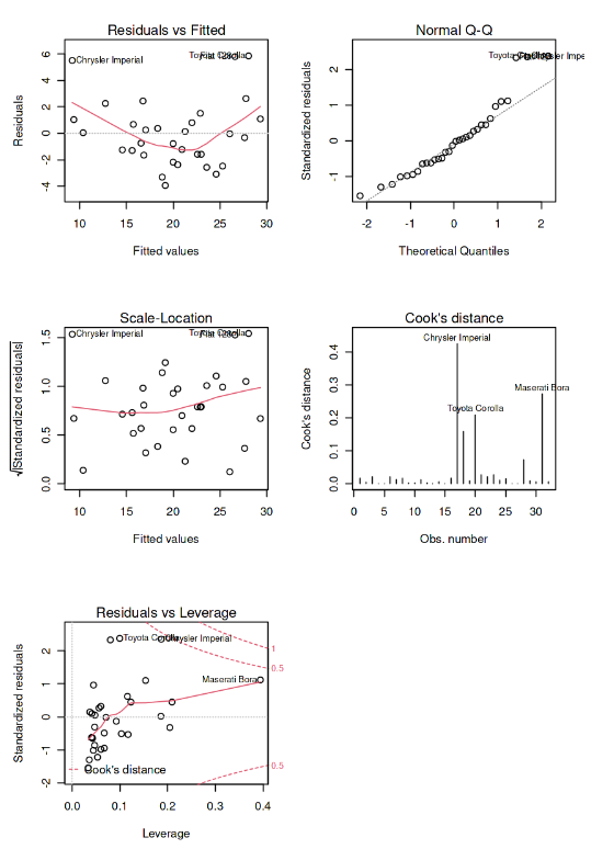
partial regression plots for the variables in the model

The above four diagnostic plots are used to check for the assumptions of linear regression models. The Residuals vs Fitted plot checks for the assumption of linearity by showing the relationship between the residuals and the fitted values. The Normal Q-Q plot checks for the assumption of normality by comparing the distribution of the residuals to a normal distribution. The Scale-Location plot checks for the assumption of homoscedasticity by showing the relationship between the square root of the standardized residuals and the fitted values. 

The Cook’s Distance plot checks for influential observations by showing the influence of each observation on the regression coefficients. These plots are important for evaluating the fit of a linear regression model and identifying potential issues, such as outliers or influential observations.

The above shows the influence of each observation on the model fit. Leverage is a measure of how much an observation differs from the average of the predictor variables. It can be used to identify potential influential observations. It suggests a well-fit linear regression model as the points in the plot are randomly distributed, with no points having both high leverage and high residuals.

Conclusion

In conclusion, the car package in R provides a variety of functions and tools for conducting regression analysis and diagnostic plots. In this tutorial, we covered examples of using the car package for regression analysis. By working through the above examples you should now have a good understanding of how to use the car package for regression analysis in R. Whether you’re a beginner or an experienced R user, the car package is a valuable tool for conducting regression analysis and exploring relationships between variables in your data.