Handle date and time columns using R

Managing date and time data is a crucial aspect of data analysis, as many datasets involve temporal information. R Programming Language is used for statistical computing and data analysis and provides several functions and packages to handle date and time columns effectively. Here we cover various techniques and tools available in R to manipulate, analyze, and visualize date and time data.

How to Handle date and time columns using R?

Handling date and time columns using R refers to the process of effectively managing and manipulating datasets that contain temporal information. R provides a set of functions and packages to load, convert, and analyze date and time data. Key tasks include converting character strings to date-time objects, performing arithmetic operations, dealing with time zones, and visualizing temporal patterns. Proper handling of date and time columns is essential for accurate analysis, forecasting, and deriving insights from time-dependent datasets.

Importance of Handling Date and Time Columns

1. Temporal Analysis: Understand patterns and trends over time.
2. Event Sequencing: Analyze chronological order of occurrences.
3. Time-Based Aggregation: Summarize and analyze data over intervals.
4. Forecasting: Build accurate models considering temporal dependencies.
5. Comparative Analysis: Compare metrics and assess changes over time.
6. Data Filtering: Easily filter and subset data based on time intervals.
7. Visualization: Create effective time series plots for insights.
8. Time Zone Handling: Ensure consistency in global datasets.
9. Data Cleaning: Address inconsistencies during cleaning and transformation.
10. Integration: Facilitate integration of diverse datasets with consistent time formats.

Popular Packages in R for Handle Date and Time

In R, several popular packages are widely used for handling date and time data, each offering unique functionalities to make working with temporal information more efficient. Some of the most popular packages and their main uses:-

1. base R functions (as.Date(), as.POSIXct())

Core functions for basic conversion of character strings to date and time objects.

2. lubridate

Simplifies working with date and time data, providing intuitive functions for common operations.

R

library(lubridate)
date_object <- ymd("2024-02-03")
date_object

Output:

[1] "2024-02-03"

3. chron

Handles dates and times as numeric values, making arithmetic operations straightforward.

R

# Load the necessary packages
library(chron)
library(lubridate)

# Create a datetime object with corrected date format
datetime_object <- chron(dates = c("02/03/2024", "02/04/2024"),
                         times = c("12:30:45", "15:20:10"))

# Display the datetime object
datetime_object

Output:

[1] (02/03/24 12:30:45) (02/04/24 15:20:10)

4.zoo

Particularly useful for irregular time series data, offering efficient tools for manipulation and analysis. we will create a data frame with two columns.

R

# Load the zoo package
library(zoo)

# Create a simple dataset
data <- data.frame(
  date_column = as.Date(c("2024-02-01", "2024-02-03", "2024-02-06")),
  value_column = c(10, 15, 20)
)

# Display the dataset
print(data)

Output:

  date_column value_column
1  2024-02-01           10
2  2024-02-03           15
3  2024-02-06           20

Now create a zoo object irregular_time_series with irregularly spaced dates and corresponding values.

R

# Ensure 'date_column' is of class Date
data$date_column <- as.Date(data$date_column)

# Create an irregular time series using zoo
irregular_time_series <- zoo(data$value_column, order.by = data$date_column)

# Display the irregular time series
print(irregular_time_series)

Output:

2024-02-01 2024-02-03 2024-02-06 
        10         15         20 

5. data.table

Efficient data manipulation package; useful for handling large datasets with date-time operations.

R

library(data.table)
dt <- data.table(date_column = as.Date(c("2024-02-03", "2024-02-04")),
                      value_column = c(10, 15))
dt

Output:

   date_column value_column
1:  2024-02-03           10
2:  2024-02-04           15

6. ggplot2

A powerful visualization package for creating time series plots.

R

library(ggplot2)
ggplot(data, aes(x = date_column, y = value_column)) +
geom_line() +
labs(title = "Time Series Plot", x = "Date", y = "Value")
labs

Output:

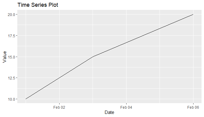
Handle date and time columns using R

These packages provide a robust set of tools for loading, manipulating, and visualizing date and time data in R.

Loading Date and Time Data

R provides the `as.Date()` and `as.POSIXct()` functions to convert character strings or numeric representations to date and time objects, respectively.

R

# Convert character string to Date
date_string <- "2024-02-03"
date_object <- as.Date(date_string)
date_object

# Convert character string to POSIXct (date and time)
datetime_string <- "2024-02-03 12:30:45"
datetime_object <- as.POSIXct(datetime_string, format="%Y-%m-%d %H:%M:%S")
datetime_object

Output:

[1] "2024-02-03"

[1] "2024-02-03 12:30:45 IST"

date_string is a character string representing a date in the format “YYYY-MM-DD” (February 3, 2024, in this case).

• as.Date() function is used to convert the character string to a Date object, and the result is stored in the variable date_object.
• date_object is then printed to the console, displaying the converted Date object.
• datetime_string is a character string representing a date and time in the format “YYYY-MM-DD HH:MM:SS” (February 3, 2024, at 12:30:45).
• as.POSIXct() function is used to convert the character string to a POSIXct (date and time) object. The format parameter specifies the expected format of the input string.
• The resulting POSIXct object is stored in the variable datetime_object.
• datetime_object is then printed to the console, displaying the converted POSIXct object.

Basic Operations with Date and Time

Once the data is loaded perform basic operations on date and time objects in R. For example, extracting components like year, month, day, hour, minute, and second can be done using various functions such as `year()`, `month()`, `day()`, `hour()`, `minute()`, and `second().

R

# Extract year, month, and day
year(date_object)
month(date_object)
day(date_object)


# Extract hour, minute, and second
hour(datetime_object)
minute(datetime_object)
second(datetime_object)

Output:

[1] 2024

[1] 2

[1] 3

[1] 12

[1] 30

[1] 45

date_object is assumed to be a Date object containing a specific date.

• year(), month(), and day() are functions provided by the lubridate package (though they are also available in base R). These functions extract the corresponding components (year, month, and day) from the Date object.
• The results are printed to the console, displaying the extracted year, month, and day.
• datetime_object is assumed to be a POSIXct object containing a specific date and time.
• hour(), minute(), and second() are functions provided by the lubridate package (though they are also available in base R). These functions extract the corresponding components (hour, minute, and second) from the POSIXct object.
• The results are printed to the console, displaying the extracted hour, minute, and second.

Date and Time Arithmetic

Performing arithmetic operations on date and time objects is common in data analysis. R allows to add or subtract days, months, or years easily.

R

date1 <- date_object + 8
date1

# Subtract 3 months from the date
date2 <- date_object - months(3)
date2
# Calculate the difference in days between two dates
time_difference <- difftime(date1, date2, units = "days")
time_difference

Output:

[1] "2024-02-11"

[1] "2023-11-03"

Time difference of 100 days

date_object is assumed to be a Date object containing a specific date.

• The – operator and the months() function (from the lubridate package) are used to subtract 3 months from the original date. The result is a new Date object stored in the variable date2.
• The value of date2 is printed to the console, displaying the result of subtracting 3 months from the original date.
• date1 and date2 are assumed to be two Date objects.
• The difftime() function is used to calculate the time difference between date1 and date2 in days. The result is stored in the variable time_difference.
• The value of time_difference is printed to the console, displaying the calculated difference in days between the two dates.

Dealing with Time Zones

Handling time zones is crucial, especially when working with data collected from different locations. The `lubridate` package provides functions like `force_tz()` and `with_tz()` for managing time zones effectively.

R

library(lubridate)

# Convert date to a specific time zone
date_with_timezone <- force_tz(date_object, tz = "America/New_York")
date_with_timezone

Output:

[1] "2024-02-03 EST"

The lubridate package is loaded, providing additional functions for handling and manipulating date and time objects.

• date_object is assumed to be a Date object containing a specific date.
• The force_tz() function from the lubridate package is used to convert the original date to a specific time zone, in this case, “America/New_York”.
• The result is a new date object with the time zone information incorporated, stored in the variable date_with_timezone.
• The value of date_with_timezone is then printed to the console, displaying the date in the specified time zone.

Working with Time Intervals

In some cases, you might need to calculate the duration between two date-time points. The `difftime()` function allows to compute time intervals in various units.

R

# Load the lubridate package for handling dates
library(lubridate)

# Create two date objects
date1 <- ymd("2024-02-15")  # February 15, 2024
date2 <- ymd("2024-01-10")  # January 10, 2024

# Calculate the time difference in days
time_difference_days <- as.numeric(date1 - date2)

# Display the result
print(paste("Time difference in days:", time_difference_days))

Output:

[1] "Time difference in days: 36"

The lubridate package is loaded, providing convenient functions for working with dates and times.

• ymd() is a function from the lubridate package that converts a character string to a Date object.
• date1 and date2 are created as Date objects representing specific dates in the year 2024.
• The – operator is used to calculate the time difference between date1 and date2.
• The as.numeric() function is then applied to convert the time difference to a numeric value, representing the difference in days.
• The result is stored in the variable time_difference_days.

Visualizing Temporal Data

Visualization is a powerful tool in understanding temporal patterns. The `ggplot2` package provides functions to create appealing time series plots.

R

# Load necessary libraries
library(ggplot2)
library(lubridate)

# Generate sample data with multiple groups
set.seed(123)
n <- 100
date_sequence <- seq(as.Date("2024-01-01"), by = "days", length.out = n)
group1_values <- cumsum(rnorm(n))
group2_values <- cumsum(rnorm(n, mean = 1))

data <- data.frame(
  date_column = rep(date_sequence, 2),
  value_column = c(group1_values, group2_values),
  group_column = rep(c("Group 1", "Group 2"), each = n)
)

# Create a time series plot with multiple lines
ggplot(data, aes(x = date_column, y = value_column, color = group_column)) +
  geom_line() +
  labs(title = "Time Series Plot with Multiple Groups", x = "Date", y = "Value") +
  theme_minimal()

Output:

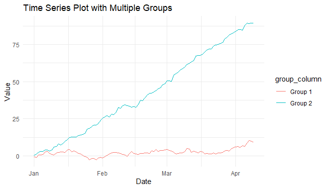
Handle date and time columns using R

We use lubridate to generate a sequence of dates (date_sequence) spanning 100 days starting from “2024-01-01”.

• We create a data frame (data) with three columns: date_column, value_column, and group_column.
• The value_column contains cumulative values for two groups generated using random numbers.
• We use ggplot2 to create a time series plot with different colors representing each group.

Advantages of Handling Date and Time in R

1. Robust Libraries:- R offers powerful date-time libraries like `lubridate` and `zoo` for extensive functionality.
2. Consistent Time Zones:- R ensures consistent time zone handling for accurate representation and conversion.
3. Effective Temporal Analysis:- R facilitates in-depth analysis, aiding trend identification and pattern recognition in time series data.
4. Efficient Filtering:- R simplifies data filtering and subsetting based on specific time intervals for targeted analysis.
5. Integration with Modeling:- R’s compatibility with statistical modeling packages enhances forecasting accuracy.
6. Time Series Visualization:- R provides visualization packages like `ggplot2` for creating informative time series plots.

Disadvantages of Handling Date and Time in R

1. Learning Curve:- Beginners may face a learning curve in mastering date-time functions and libraries in R.
2. Computational Overhead:- Some date-time operations in R may have computational overhead, impacting performance with large datasets.
3. Handling Complexity:- Managing date-time data involving leap years or time zone changes requires careful attention.
4. Ambiguity Risks:- Misinterpretation of date formats can lead to errors, emphasizing the need for consistent formatting.
5. Dependency on Libraries:- Some advanced date-time functionality depends on external libraries like `lubridate`, requiring correct installation and updates.
6. Limited Plot Customization:- R provides effective time series plotting, but there might be limitations in customization compared to specialized tools.

Practical Application

1. Financial Analytics:- Analyzing stock prices, market trends, and economic indicators over time.
2. Healthcare Analytics:- Tracking patient records, monitoring treatment effectiveness, and analyzing medical outcomes.
3. E-commerce and Marketing:- Analyzing user behavior, tracking sales patterns, and optimizing marketing campaigns over time.
4. Energy Consumption Analysis:- Monitoring and optimizing energy usage patterns to enhance efficiency.
5. Supply Chain Management:- Tracking inventory levels, delivery times, and optimizing supply chain operations.
6. Web Analytics:- Analyzing website traffic patterns, user engagement, and behavior over time.
7. Predictive Maintenance:- Predicting equipment failures and scheduling maintenance based on historical data.
8. Climate and Environmental Studies: – Analyzing climate data, tracking environmental changes, and studying long-term trends.
9. Human Resources Management: – Managing employee attendance, tracking performance metrics, and analyzing workforce trends.
10. Traffic and Transportation Management:- Analyzing traffic patterns, optimizing routes, and improving transportation systems.

Conclusion

Handling of date and time in R equips data analysts with essential skills for effective data manipulation, analysis, and visualization. The availability of robust libraries such as `lubridate` and `zoo` enables seamless operations, from basic conversions to advanced time series analysis. The significance of proper date and time handling is evident in its applications across diverse fields, ranging from financial analytics to healthcare and beyond. While R offers powerful tools, users must navigate potential challenges, including a learning curve and dependencies on external libraries. Overall, the ability to handle date and time in R proves indispensable for deriving meaningful insights from time-dependent datasets and making informed decisions.