What is Perceptron | The Simplest Artificial neural network

Last Updated : 28 Nov, 2023

A single-layer feedforward neural network was introduced in the late 1950s by Frank Rosenblatt. It was the starting phase of Deep Learning and Artificial neural networks. During that time for prediction, Statistical machine learning, or Traditional code Programming is used. Perceptron is one of the first and most straightforward models of artificial neural networks. Despite being a straightforward model, the perceptron has been proven to be successful in solving specific categorization issues.

What is Perceptron?

Perceptron is one of the simplest Artificial neural network architectures. It was introduced by Frank Rosenblatt in 1957s. It is the simplest type of feedforward neural network, consisting of a single layer of input nodes that are fully connected to a layer of output nodes. It can learn the linearly separable patterns. it uses slightly different types of artificial neurons known as threshold logic units (TLU). it was first introduced by McCulloch and Walter Pitts in the 1940s.

Types of Perceptron

Single-Layer Perceptron: This type of perceptron is limited to learning linearly separable patterns. effective for tasks where the data can be divided into distinct categories through a straight line.
Multilayer Perceptron: Multilayer perceptrons possess enhanced processing capabilities as they consist of two or more layers, adept at handling more complex patterns and relationships within the data.

Basic Components of Perceptron

A perceptron, the basic unit of a neural network, comprises essential components that collaborate in information processing.

Input Features: The perceptron takes multiple input features, each input feature represents a characteristic or attribute of the input data.
Weights: Each input feature is associated with a weight, determining the significance of each input feature in influencing the perceptron’s output. During training, these weights are adjusted to learn the optimal values.
Summation Function: The perceptron calculates the weighted sum of its inputs using the summation function. The summation function combines the inputs with their respective weights to produce a weighted sum.
Activation Function: The weighted sum is then passed through an activation function. Perceptron uses Heaviside step function functions. which take the summed values as input and compare with the threshold and provide the output as 0 or 1.
Output: The final output of the perceptron, is determined by the activation function’s result. For example, in binary classification problems, the output might represent a predicted class (0 or 1).
Bias: A bias term is often included in the perceptron model. The bias allows the model to make adjustments that are independent of the input. It is an additional parameter that is learned during training.
Learning Algorithm (Weight Update Rule): During training, the perceptron learns by adjusting its weights and bias based on a learning algorithm. A common approach is the perceptron learning algorithm, which updates weights based on the difference between the predicted output and the true output.

These components work together to enable a perceptron to learn and make predictions. While a single perceptron can perform binary classification, more complex tasks require the use of multiple perceptrons organized into layers, forming a neural network.

How does Perceptron work?

A weight is assigned to each input node of a perceptron, indicating the significance of that input to the output. The perceptron’s output is a weighted sum of the inputs that have been run through an activation function to decide whether or not the perceptron will fire. it computes the weighted sum of its inputs as:

z = w₁x₁ + w₁x₂ + ... + w_nx_n = X^TW

The step function compares this weighted sum to the threshold, which outputs 1 if the input is larger than a threshold value and 0 otherwise, is the activation function that perceptrons utilize the most frequently. The most common step function used in perceptron is the Heaviside step function:

A perceptron has a single layer of threshold logic units with each TLU connected to all inputs.

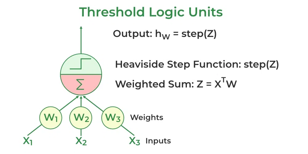
Threshold Logic units

When all the neurons in a layer are connected to every neuron of the previous layer, it is known as a fully connected layer or dense layer.

The output of the fully connected layer can be:

where X is the input W is the weight for each inputs neurons and b is the bias and h is the step function.

During training, The perceptron’s weights are adjusted to minimize the difference between the predicted output and the actual output. Usually, supervised learning algorithms like the delta rule or the perceptron learning rule are used for this.

Here w_i,j is the weight between the ith input and jth output neuron, x_i is the ith input value, and y_j and $\hat y_j$ is the jth actual and predicted value is $\eta$ the learning rate.

Implementations code

Build the single Layer Perceptron Model

Initialize the weight and learning rate, Here we are considering the weight values number of input + 1. i.e +1 for bias.
Define the first linear layer
Define the activation function. Here we are using the Heaviside Step function.
Define the Prediction
Define the loss function.
Define training, in which weight and bias are updated accordingly.
define fitting the model.

Python3

# Import the necessary library
import numpy as np
 
# Build the Perceptron Model
class Perceptron:
     
    def __init__(self, num_inputs, learning_rate=0.01):
        # Initialize the weight and learning rate
        self.weights = np.random.rand(num_inputs + 1)
        self.learning_rate = learning_rate
     
    # Define the first linear layer 
    def linear(self, inputs):
        Z = inputs @ self.weights[1:].T + + self.weights[0]
        return Z
     
    # Define the Heaviside Step function.
    def Heaviside_step_fn(self, z):
        if z >= 0:
            return 1
        else:
            return 0
         
    # Define the Prediction
    def predict(self, inputs):
        Z = self.linear(inputs)
        try:
            pred = []
            for z in Z:
                pred.append(self.Heaviside_step_fn(z))
        except:
            return self.Heaviside_step_fn(Z)
        return pred
     
    # Define the Loss function
    def loss(self, prediction, target):
        loss = (prediction-target)
        return loss
     
    #Define training
    def train(self, inputs, target):
        prediction = self.predict(inputs)
        error = self.loss(prediction, target)
        self.weights[1:] += self.learning_rate * error * inputs
        self.weights[0]  += self.learning_rate * error
         
    # Fit the model
    def fit(self, X, y, num_epochs):
        for epoch in range(num_epochs):
            for inputs, target in zip(X, y):
                self.train(inputs, target)

Apply the above-defined model for binary classification of the Breast Cancer Dataset

import the necessary libraries
Load the dataset
Assign the input features to x
Assign the target features to y
Initialize the Perceptron with the appropriate number of inputs
Train the model
Predict from the test dataset
Find the accuracy of the model

Python3

# Import the necessary library
import numpy as np
from sklearn.datasets import make_blobs
import matplotlib.pyplot as plt
from sklearn.model_selection import train_test_split
from sklearn.preprocessing import StandardScaler
 
# Generate a linearly separable dataset with two classes
X, y = make_blobs(n_samples=1000,
                  n_features=2, 
                  centers=2, 
                  cluster_std=3,
                  random_state=23)
 
# Split the dataset into training and testing sets
X_train, X_test, y_train, y_test = train_test_split(X,
                                                    y,
                                                    test_size=0.2,
                                                    random_state=23,
                                                    shuffle=True
                                                   )
 
# Scale the input features to have zero mean and unit variance
scaler = StandardScaler()
X_train = scaler.fit_transform(X_train)
X_test = scaler.transform(X_test)
 
# Set the random seed legacy
np.random.seed(23)
 
# Initialize the Perceptron with the appropriate number of inputs
perceptron = Perceptron(num_inputs=X_train.shape[1])
 
# Train the Perceptron on the training data
perceptron.fit(X_train, y_train, num_epochs=100)
 
# Prediction
pred = perceptron.predict(X_test)
 
# Test the accuracy of the trained Perceptron on the testing data
accuracy = np.mean(pred != y_test)
print("Accuracy:", accuracy)
 
# Plot the dataset
plt.scatter(X_test[:, 0], X_test[:, 1], c=pred)
plt.xlabel('Feature 1')
plt.ylabel('Feature 2')
plt.show()

Output:

Accuracy: 0.975

Classification Result

Build and train the single Layer Perceptron Model in Pytorch

Python3

# Import the necessary libraries
import torch
import torch.nn as nn
from sklearn.datasets import make_blobs
import matplotlib.pyplot as plt
from sklearn.model_selection import train_test_split
from sklearn.preprocessing import StandardScaler
 
# Generate a linearly separable dataset with two classes
X, y = make_blobs(n_samples=1000,
                  n_features=2, 
                  centers=2, 
                  cluster_std=3,
                  random_state=23)
 
# Split the dataset into training and testing sets
X_train, X_test, y_train, y_test = train_test_split(X,
                                                    y,
                                                    test_size=0.2,
                                                    random_state=23,
                                                    shuffle=True
                                                   )
 
# Scale the input features to have zero mean and unit variance
scaler = StandardScaler()
X_train = scaler.fit_transform(X_train)
X_test = scaler.transform(X_test)
 
# Convert the data to PyTorch tensors
X_train = torch.tensor(X_train, dtype=torch.float32, requires_grad=False)
X_test = torch.tensor(X_test, dtype=torch.float32, requires_grad=False)
y_train = torch.tensor(y_train, dtype=torch.float32, requires_grad=False)
y_test = torch.tensor(y_test, dtype=torch.float32, requires_grad=False)
 
# reshape the target tensor to match the predicted output tensor
y_train = y_train.reshape(-1, 1)
y_test = y_test.reshape(-1, 1)
 
torch.random.seed()
 
# Define the Perceptron model
class Perceptron(nn.Module):
    def __init__(self, num_inputs):
        super(Perceptron, self).__init__()
        self.linear = nn.Linear(num_inputs, 1)
         
    # Heaviside Step function
    def heaviside_step_fn(self,Z):
        Class = []
        for z in Z:
            if z >= 0:
                Class.append(1)
            else:
                Class.append(0)
        return torch.tensor(Class)
     
    def forward(self, x):
        Z = self.linear(x)
        return self.heaviside_step_fn(Z)
         
 
# Initialize the Perceptron with the appropriate number of inputs
perceptron = Perceptron(num_inputs=X_train.shape[1])
 
# loss function
def loss(y_pred,Y):
    cost = y_pred-Y
    return cost
 
 
# Learning Rate
learning_rate = 0.001
 
# Train the Perceptron on the training data
num_epochs = 10
for epoch in range(num_epochs):
    Losses = 0
    for Input, Class in zip(X_train, y_train):
        # Forward pass
        predicted_class = perceptron(Input)
        error = loss(predicted_class, Class)
        Losses += error
        # Perceptron Learning Rule
 
        # Model Parameter
        w = perceptron.linear.weight
        b = perceptron.linear.bias
 
        # Matually Update the model parameter
        w = w - learning_rate * error * Input
        b = b - learning_rate * error
 
        # assign the weight & bias parameter to the linear layer
        perceptron.linear.weight = nn.Parameter(w)
        perceptron.linear.bias   = nn.Parameter(b)
    print('Epoch [{}/{}], weight:{}, bias:{} Loss: {:.4f}'.format(
        epoch+1,num_epochs,
        w.detach().numpy(),
        b.detach().numpy(),
        Losses.item()))
 
# Test the accuracy of the trained Perceptron on the testing data
pred = perceptron(X_test)
 
accuracy = (pred==y_test[:,0]).float().mean()
print("Accuracy on Test Dataset:", accuracy.item())
     
# Plot the dataset
plt.scatter(X_test[:, 0], X_test[:, 1], c=pred)
plt.xlabel('Feature 1')
plt.ylabel('Feature 2')
plt.show()

Output:

Epoch [1/10], weight:[[ 0.01072957 -0.7055903 ]], bias:[0.07482227] Loss: 4.0000
Epoch [2/10], weight:[[ 0.0140219  -0.70487624]], bias:[0.07082226] Loss: 4.0000
Epoch [3/10], weight:[[ 0.0175706  -0.70405596]], bias:[0.06782226] Loss: 3.0000
Epoch [4/10], weight:[[ 0.02111931 -0.7032357 ]], bias:[0.06482225] Loss: 3.0000
Epoch [5/10], weight:[[ 0.02466801 -0.7024154 ]], bias:[0.06182225] Loss: 3.0000
Epoch [6/10], weight:[[ 0.02821671 -0.7015951 ]], bias:[0.05882225] Loss: 3.0000
Epoch [7/10], weight:[[ 0.03176541 -0.70077485]], bias:[0.05582226] Loss: 3.0000
Epoch [8/10], weight:[[ 0.03479535 -0.69990206]], bias:[0.05382226] Loss: 2.0000
Epoch [9/10], weight:[[ 0.03782528 -0.69902927]], bias:[0.05182226] Loss: 2.0000
Epoch [10/10], weight:[[ 0.04085522 -0.6981565 ]], bias:[0.04982227] Loss: 2.0000
Accuracy on Test Dataset: 0.9900000095367432

Classification Result

Limitations of Perceptron

The perceptron was an important development in the history of neural networks, as it demonstrated that simple neural networks could learn to classify patterns. However, its capabilities are limited:

The perceptron model has some limitations that can make it unsuitable for certain types of problems:

Limited to linearly separable problems.
Convergence issues with non-separable data
Requires labeled data
Sensitivity to input scaling
Lack of hidden layers

More complex neural networks, such as multilayer perceptrons (MLPs) and convolutional neural networks (CNNs), have since been developed to address this limitation and can learn more complex patterns.

Frequently Asked Questions(FAQs)

1. What is the Perceptron model in Machine Learning?

The perceptron is a linear algorithm in machine learning employed for supervised learning tasks involving binary classification. It serves as a foundational element for understanding both machine learning and deep learning, comprising weights, input values or scores, and a threshold.

2. What is Binary classifier in Machine Learning?

A binary classifier in machine learning is a type of algorithm designed to categorize input data into two distinct classes or categories. The goal is to assign each input instance to one of the two classes based on its features or characteristics.

3. What are the basic components of Perceptron?

The basic components of a perceptron include input values or features, weights associated with each input, a summation function, an activation function, a bias term, and an output. These elements collectively enable the perceptron to learn and make binary classifications in machine learning tasks.

4. What is the Perceptron Learning Algorithm?

The Perceptron Learning Algorithm is a binary classification algorithm used in supervised learning. It adjusts weights associated with input features iteratively based on misclassifications, aiming to find a decision boundary that separates classes. It continues until all training examples are correctly classified or a predefined number of iterations is reached.

5. What is the difference between Perceptron and Multi-layer Perceptron?

The Perceptron is a single-layer neural network used for binary classification, learning linearly separable patterns. In contrast, a Multi-layer Perceptron (MLP) has multiple layers, enabling it to learn complex, non-linear relationships. MLPs have input, hidden, and output layers, allowing them to handle more intricate tasks compared to the simpler Perceptron.

Suggest improvement

Artificial Neural Network in TensorFlow

Share your thoughts in the comments

What is Perceptron | The Simplest Artificial neural network