Artificial Neural Network in TensorFlow

In this article, we are going to see some basics of ANN and a simple implementation of an artificial neural network. Tensorflow is a powerful machine learning library to create models and neural networks.

So, before we start What are Artificial neural networks? Here is a simple and clear definition of artificial neural networks. So long story in short artificial neural networks is a technology that mimics a human brain to learn from some key features and classify or predict in the real world. An artificial neural network is composed of numbers of neurons which is compared to the neurons in the human brain.  

It is designed to make a computer learn from small insights and features and make them autonomous to learn from the real world and provide solutions in real-time faster than a human.

A neuron in an artificial neural network, will perform two operations inside it

• Sum of all weights
• Activation function

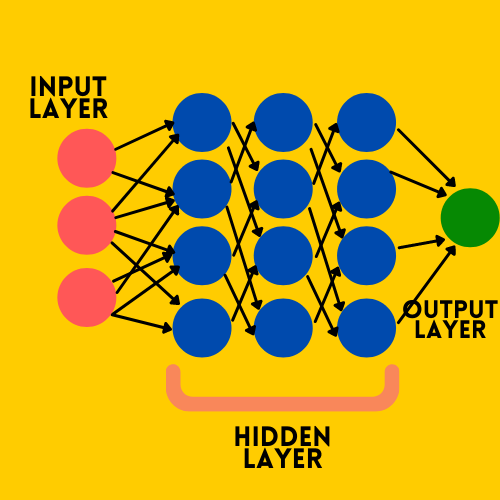
So a basic Artificial neural network will be in a form of,

1. Input layer – To get the data from the user or a client or a server to analyze and give the result.
2. Hidden layers – This layer can be in any number and these layers will analyze the inputs with passing through them with different biases, weights, and activation functions to provide an output
3. Output Layer – This is where we can get the result from a neural network.

So as we know the outline of the neural networks, now we shall move to the important functions and methods that help a neural network to learn correctly from the data.  

Note: Any neural network can learn from the data but without good parameter values a neural network might not able to learn from the data correctly and will not give you the correct result.

Some of the features that determine the quality of our neural network are:

1. Layers
2. Activation function
3. Loss function
4. Optimizer

Now we shall discuss each one of them in detail, 

The first stage of our model building is:

Python3

# Defining the model
model = keras.Sequential([
    keras.layers.Dense(32, input_shape=(2,), activation='relu'),
    keras.layers.Dense(16, activation = 'relu'),
    keras.layers.Dense(2, activation = 'sigmoid')
])

Layers

Layers in a neural network are very important as we saw earlier an artificial neural network consists of 3 layers an input layer, hidden layer, output layer. The input layer consists of the features and values that need to be analyzed inside a neural network. Basically, this is a layer that will read our input features onto an Artificial neural network.

A hidden layer is a layer where all the magic happens when all the input neurons pass the features to the hidden layer with a weight and a bias each and every neuron inside the hidden layer will sum up all the weighted features from all the input layers and apply an activation function to keep the values between 0 and 1 for easier learning. Here we need to choose the number of neurons in each layer manually and it must be the best value for the network.

Here the real decision-makers are the weights between each layer which will finally pass a value of 0 to 1 to the output layer. Till this, we have seen the importance of each level of layers in an artificial neural network. There are many types of layers in TensorFlow but the one that we will use a lot is Dense

syntax: tf.keras.layers.Dense()

This is a fully connected layer in which each and every feature input will be connected somehow with the result.

Activation function

Activation functions are simply mathematical methods that bring all the values inside a range of 0 to 1 so that it will be very easier for the machine to learn the data in its process of analyzing the data. There are a variety of activation functions that are supported by the Tensor flow. Some of the commonly used functions are,

1. Sigmoid
2. Relu
3. Softmax
4. Swish
5. Linear

Each and every activation function has its own specific use cases and drawbacks. But the activation function that is used in the hidden and input layers is ‘Relu’ and another this which will have a greater impact on the result is losses.

After this, we can see the params in the compilation of the model in TensorFlow,

Python

# Compilation of model
model.compile(optimizer='adam'
              loss=a_loss_function
              metrics=['metrics'])

Losses

Loss functions are a very important thing to notice while creating a neural network because loss functions in the neural network will calculate the difference between the predicted output and the actual result and greatly help the optimizers in the neural nets to update the weights on its backpropagation.

There are many loss functions that were supported by the TensorFlow library, and again commonly used few are,

1. Mean Absolute
2. MeanSquaredError
3. Binary Crossentropy
4. Categorical Crossentropy
5. Sparse Categorical Crossentropy

Note: Again the choice of loss is completely dependent on the type of problem and result we expect from the Neural network.

Optimizers

Optimizers are a very important thing because this is the function that helps the neural network to change the weights on the backpropagation so that the difference between the actual and predicted result will decrease at a gradual pace and obtain that point where the loss is very minimum and the model is able to predict more accurate results.

Again TensorFlow supports many optimizers to mention a few,

1. Gradient descent
2. SDG – Stochastic Gradient Descent
3. Adagrad
4. Adam

After compiling the model we need to fit the model with the dataset for training,

Python

# fitting the model
model.fit(train_data, train_label,
          epochs=5, batch_size=32)

Epochs

Epochs are simply the number of times the entire dataset passes forward and backpropagated by updating the weights on a neural network. BY doing this we can find unseen patterns and information in every single epoch and hence it improves the accuracy of the model.

And to handle some limitations of the neural networks like overfitting the training data and could not able to perform well on the unseen data. This can be solved by some dropout layers which means making some amount of nodes in a layer inactive which forces each and every node in the neural network to learn more about the features of the input and hence the problem can be solved. 

In TensorFlow, to add a dropout in a layer is literally a line of code,

syntax: tf.keras.layers.Dropout(rate, noise_shape=None, seed=None, **kwargs )

How to Train a Neural Network with TensorFlow :

Step 1: Importing the libraries

We are going to import the required libraries.

Python

# Importing the libraries
import pandas as pd
import numpy as np
from tensorflow import keras
from tensorflow.keras import layers
from sklearn.model_selection import train_test_split

Step 2: Importing the data

The data we used for this example are generated randomly with Numpy. In this data x and y are the point of coordinates and the color feature is the target value that was generated randomly which is in binary representing Red – 1 , Blue – 0.

Python

# Importing the data
df = pd.read_csv('data.txt')

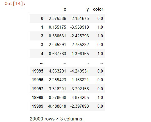
The data will look like:

Step 3: Splitting the data

Now we are going to split the dataset into train and test splits to evaluate the model with the unseen data and check its accuracy.

Python

# split the data into train and test set
train, test = train_test_split(
    df, test_size=0.2, random_state=42, shuffle=True)

Step 4: Constructing the input

In this step, we are going to construct the input we need to feed into a network. For simplicity and for the model’s sake we are going to stack the two features of the data into x and the target variable as y. We use numpy.column_stack() to stack the 

Python

# Constructing the input
x = np.column_stack((train.x.values, train.y.values))
y = train.color.values

Step 5: Building a model

Now we are going to build a simple neural network to classify the color of the point with two input nodes and a hidden layer and an output layer with relu and sigmoid activation functions, and sparse categorical cross-entropy loss function and this is going to be a fully connected feed-forward network.

Python

# Defining the model
model = keras.Sequential([
    keras.layers.Dense(4, input_shape=(2,), activation='relu'),
    keras.layers.Dense(2, activation='sigmoid')
])

# Compiling the model
model.compile(optimizer='adam',
              loss=keras.losses.SparseCategoricalCrossentropy(),
              metrics=['accuracy'])

# fitting the model
model.fit(x, y, epochs=10, batch_size=8)

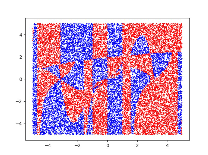
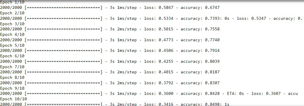
Output:

If we evaluate the model with unseen data it will give a very low amount of accuracy,

Python

# Evaluating the model
x = np.column_stack((test.x.values, test.y.values))
y = test.color.values
model.evaluate(x, y, batch_size=8)

Step 6: Building a better model

Now we are going to improve the model with a few extra hidden layers and a better activation function ‘softmax’ in the output layer and built a better neural network.

Python

# Defining the model
model_better = keras.Sequential([
    keras.layers.Dense(16, input_shape=(2,), activation='relu'),
    keras.layers.Dense(32, activation='relu'),
    keras.layers.Dense(32, activation='relu'),
    keras.layers.Dense(2, activation='softmax')
])

# Compiling the model
model_better.compile(optimizer='adam',
                     loss=keras.losses.SparseCategoricalCrossentropy(),
                     metrics=['accuracy'])

# Constructing the input
x = np.column_stack((train.x.values, train.y.values))
y = train.color.values

# fitting the model
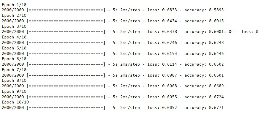
model_better.fit(x, y, epochs=10, batch_size=8)

Output:

Step 7: Evaluating the model

Finally, if we evaluate the model we can clearly see that the accuracy of the model on unseen data has been improved from 66 -> 85. So we built an efficient model.