Using Colors to Create Engaging Visualisations in R

Colors are an effective medium for communicating information. The color display of data plays a critical role in visualization and exploratory data analysis. The exact use of color for data display allows for known interrelationships and patterns within data. The careless use of color will create uncertain patterns so, it becomes difficult to understand. The main part of data analysis is storytelling, using colors in storytelling helps stack holders understand the dashboard easily. Appropriate use of colors is used to make effective data-driven decisions.    

Use colors to create engaging visuals in R

We have to use colors to create good quality visuals so, that make sense to the viewer. It helps viewers and stack holders to understand the information faster and more effectively. Color plays a significant role in data visualization. Viewers need to understand the report easily so if we highlight certain pieces of information and promote information recall it will be easy for viewers to understand the report created by analysts. Using colors strategically can aid pattern recognition and attract attention to important information and this is exactly what we will be looking at in this article using R.

Some rules to follow while using colors

• Use a single color to represent continuous data.
• Use contrasting colors to represent a comparison between columns.
• Use colors to make important data stand out.
• Use limited colors. Too many colors in a single dashboard lead to ambiguity.
• Use the correct graph style and coloring for your data.

To demonstrate the color usage in plots we will be using the Palmer Penguins dataset which has 8 attributes and 344 observations throughout this article. Penguins’ data set gives complete information about penguins’ bodies.

R

# install packages
install.packages("dplyr")
install.packages("palmerpenguins")

# load packages
library(dplyr)
library(palmerpenguins)

# summary of penguins dataset
summary(penguins)

Output:

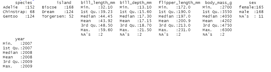
Summary of the penguin dataset

Using default Colors with ggplot

When we draw some visualization using ggplot2 package the default colors are provided by the library to distinguish between different categories present in the data provided for visualization.

R

# load packages
install.packages("ggplot2")
library(ggplot2)

# data layer + Geometric layer + Aesthetics layer
ggplot(data = penguins) + geom_bar(mapping =
                aes(x=bill_length_mm, fill = species))

Output:

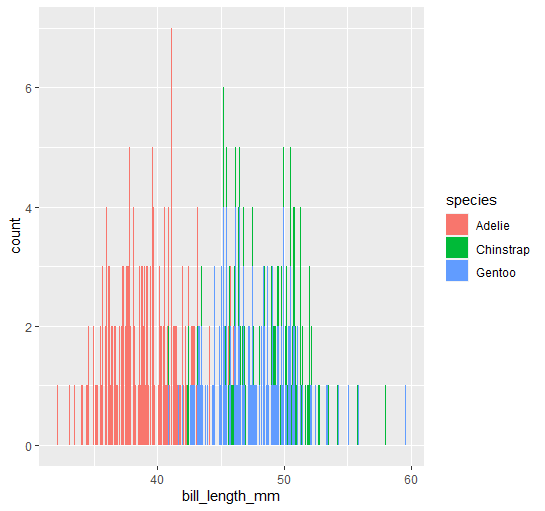
Plot with default colors

If we use a bar chart for each penguin of different bill_length and bill_depth we cannot get clear data so, using the right graph is important along with colors below is an example of good usage of a suitable graph and colors. Also, one thing that we can observe in the below graph is that the colors used are the same as that present in the previous visualization this makes an analysis report boring and less comprehensive.

R

# load packages
library(ggplot2)

# data layer + Geometric layer + Aesthetics layer
ggplot(data = penguins) + geom_point(mapping =
          aes(x=bill_length_mm, y=bill_depth_mm, col = species))

Output:

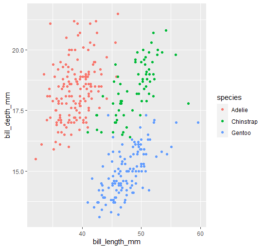
The different plot formed using ggplot with the same colors

We generally use col aesthetic to use colors in our visuals in the case of a bar graph col aesthetic does not give color variation it just outlines the bar in a bar chart so, for this problem we use the fill attribute to replace of cool aesthetic.

R

#install and load packages if you are using new R script
age <- c(19,34,56,23,45,18,34,32,17,15,16,9)
gender <- c("f","f","m","f","m","m","m","f","m","m","f","m")
height_in_cm <- c(183.98,178.56,167.984,156.78,178.35,145.78,190.23,167.23,156.278,178.89,189.56,130.90)
people <- data.frame(age, gender, height_in_cm)
ggplot(data = people) + geom_line(mapping = aes(x = height_in_cm, y = age, col = gender))

Output:

Wes Anderson package to Create Engaging Visualizations in R

There are also some inbuilt color palettes in R language these palettes are available in the Wes Anderson package. Install Wes Anderson package in R script to access available color palettes in R language.

Syntax:

wes_palette(name, n, type = c(“discrete”, “continuous”))

Parameters:

• name – Name of the color Palette
• n – Number of colors desired
• type
  • Discrete
  • Continuous

Some of the color palettes available in the Wes Anderson are as shown below:

• Royal1
• Cavalcanti1
• GrandBudapest1
• Moonrise1
• FantasticFox1

Let’s start with the installation of this package.

R

# install package wesanderson
install.packages("wesanderson")
library(wesanderson)

Now we will draw some palettes and use them further to make visualizations. The first palette that we will be looking at is Royal1.

R

wes_palette("Royal1")

Output:

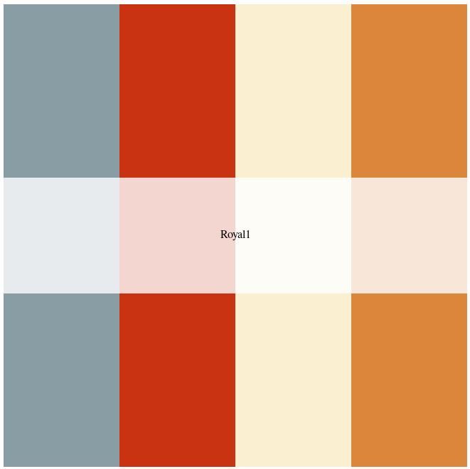
Royal1 color palette in Wes Anderson package

Now let’s make a visualization using this Royal1 color palette.

R

monochromatic <- ggplot(penguins, aes(x = bill_length_mm,
                                      y = bill_depth_mm,
                                      color = species)) +
                                        geom_point(stat = "identity")

# Royal1 is a available palette name
monochromatic +
scale_color_manual(values = wes_palette(n=3,
                                        name = "Royal1"))

Output:

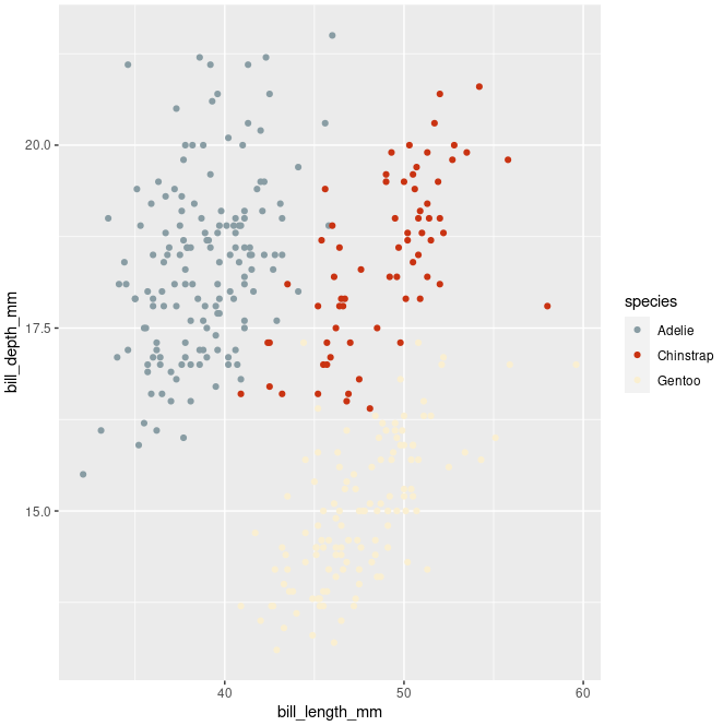
Plot using Royal1 Color Palette

Now let’s look at the Cavalcanti1 color palettes.

R

wes_palette("Cavalcanti1")

Output:

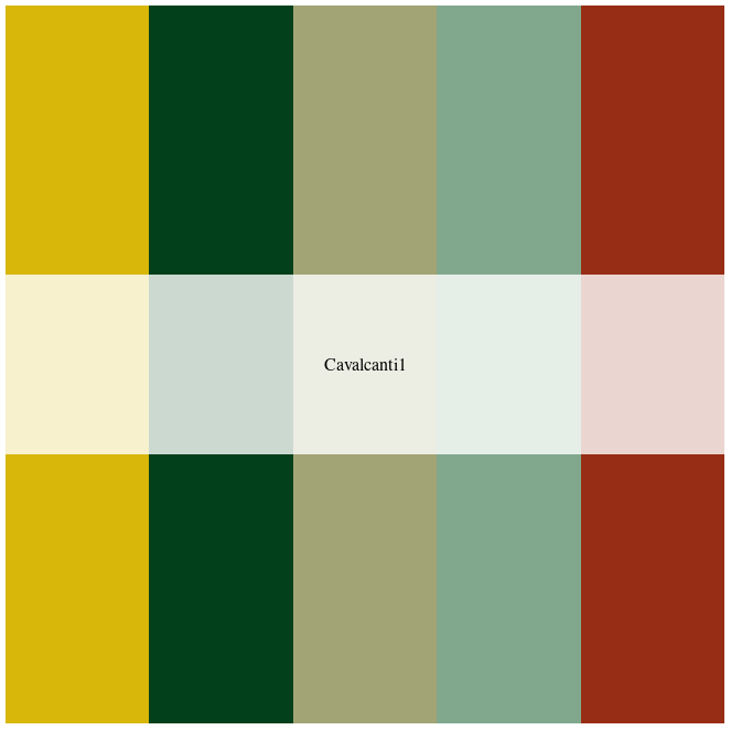
Cavalcanti1 Color Palette

Now let’s make a visualization using this Cavalcanti1 color palette.

R

cavalcanti <- ggplot(penguins, aes(x = species,
                                   y = body_mass_g,
                                   fill = species)) + geom_bar(stat = "identity")

# cavalcanti is a available palette name
cavalcanti +
scale_color_manual(values = wes_palette(n=3,
                                        name = "Cavalcanti1"))

Output:

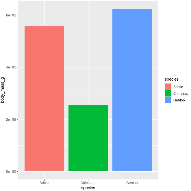
Plot using Cavalcanti1 Color Palette

RColorBrewer package to Create Engaging Visualizations in R

Another package we can use for creating good visualizations in R is using RColorBrewer. This package creates good-looking color palettes for visualization. To know more about the RColorBrewer package. This article also covers different types of color palettes like Sequential, Diverging, and Qualitative color palettes.

R

# install and load RColorBrewer
install.packages("RColorBrewer")
library(RColorBrewer)

We can list all the colors with their key information using brewer.pal.info.

R

brewer.pal.info

Output:

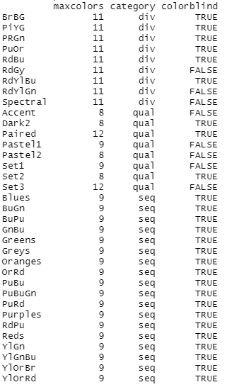
Different palettes available in RColorBrewer Package

Functions in RColorBrewer

Below are some of the built-in functions which come in very handy while using the RColorBrewer package to fill colors in the visualizations we make in the process of analysis.

Function	Description
brewer.pal(n, name)	makes the color palettes from ColorBrewer available as R color palettes
display.the brewer.pal(n, name)	display the selected palettes in the R window
display.brewer.all(n, type, colorblindFriendly)	displays the few palettes simultaneously in an R window
brewer.pal.info	returns information about all available palettes as a data frame. brewer.pal.info is not a function it is a variable
scale_fill_brewer()	Used to color for bar plot, box plot, violin plot, dot plot
scale_color_brewer()	User to color for lines and points

Arguments for Functions in RColorBrewer

To obtain different results with the same functions we can pass different types of arguments as well which can help us to obtain results as per our requirement.

Arguments	Description
n	Number of different colors in the palette, minimum 3, maximum depending on the palette
name	A palette name from the available palettes
type	used to specify the type of palette using the string “div”, “qual”, “seq”, or “all”
select	A list of names of existing palettes
exact.n	If TRUE, only display palettes with a color number given by n
colorblind-friendly	If TRUE, display only colorblind-friendly palettes

To get info about any particular color palette we can use the display.brewer.pal function to display a grid with strips of different colors that are included in that particular palette.

R

# display specific R color brewer palette
display.brewer.pal(n = 8, name = 'Dark2')

Output:

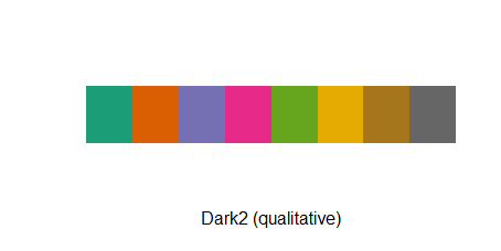
Dark2 color palette in RColorBrewer Package

We can also print the hexadecimal codes for the respective color palettes.

R

# return hexadecimal code of color palette
brewer.pal(n = 8, name = 'RdBu')

Output:

"#B2182B" "#D6604D" "#F4A582" "#FDDBC7" "#D1E5F0" "#92C5DE" "#4393C3" "#2166AC"

Now let’s see some of the color palettes in action. First, we will try the Dark2 color palette in the below visualization.

R

temp <- ggplot(data=penguins) + geom_point(mapping = aes(x = bill_length_mm,
                                                         y = bill_depth_mm,
                                                         col = species))
temp + scale_color_brewer(palette = 'Dark2')

Output:

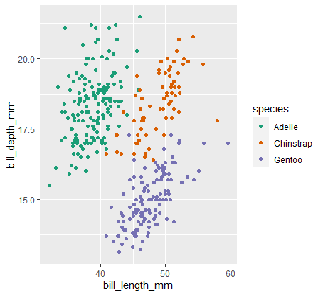
Exemplary plot with Dark2 Color Palette

Now, we will try the Greens color palette in the below visualization.

R

temp <- ggplot(data=penguins) + geom_point(mapping = aes(x = bill_length_mm,
                                                          y = bill_depth_mm,
                                                          col = species))
temp + scale_color_brewer(palette = 'Greens')

Output:

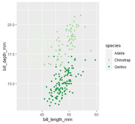
Exemplary plot with Greens Color Palette

Now, we will try the RdGy color palette in the below visualization.

R

temp <- ggplot(data=penguins) + geom_point(mapping = aes(x = bill_length_mm,
                                                         y = bill_depth_mm,
                                                         col = species))
temp + scale_color_brewer(palette = 'RdGy')

Output:

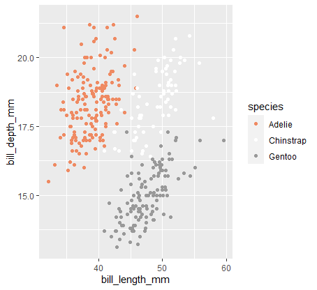
Exemplary plot with RdGy Color Palette