scipy stats.beta() | Python
Last Updated :
20 Mar, 2019
scipy.stats.beta() is an beta continuous random variable that is defined with a standard format and some shape parameters to complete its specification.
Parameters :
q : lower and upper tail probability
a, b : shape parameters
x : quantiles
loc : [optional] location parameter. Default = 0
scale : [optional] scale parameter. Default = 1
size : [tuple of ints, optional] shape or random variates.
moments : [optional] composed of letters [‘mvsk’]; ‘m’ = mean, ‘v’ = variance, ‘s’ = Fisher’s skew and ‘k’ = Fisher’s kurtosis. (default = ‘mv’).
Results : beta continuous random variable
Code #1 : Creating beta continuous random variable
from scipy.stats import beta
numargs = beta.numargs
[a, b] = [0.6, ] * numargs
rv = beta(a, b)
print ("RV : \n", rv)
|
Output :
RV :
 <scipy.stats._distn_infrastructure.rv_frozen object at 0x0000029482FCC438>
Code #2 : beta random variates and probability distribution function.
import numpy as np
quantile = np.arange (0.01, 1, 0.1)
R = beta.rvs(a, b, scale = 2, size = 10)
print ("Random Variates : \n", R)
R = beta.pdf(quantile, a, b, loc = 0, scale = 1)
print ("\nProbability Distribution : \n", R)
|
Output :
Random Variates :
 [1.47189604 1.47284574 1.84692416 1.0686604  0.32709236 1.96857076
 0.00639731 1.97093898 1.34811881 0.34269426]

Probability Distribution :
 [2.62281037 1.04883674 0.84934164 0.76724957 0.73040985 0.72096547
 0.73529768 0.77903762 0.8752367  1.1264383 ]
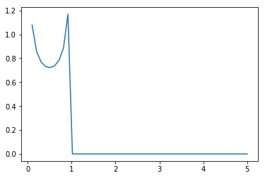
Code #3 : Graphical Representation.
import numpy as np
import matplotlib.pyplot as plt
distribution = np.linspace(0, np.maximum(rv.dist.b, 5))
plot = plt.plot(distribution, rv.pdf(distribution))
|
Output :
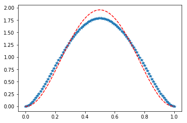
Code #4 : Varying Positional Arguments
from scipy.stats import arcsine
import matplotlib.pyplot as plt
import numpy as np
x = np.linspace(0, 1.0, 100)
y1 = beta.pdf(x, 2.75, 2.75)
y2 = beta.pdf(x, 3.25, 3.25)
plt.plot(x, y1, "*", x, y2, "r--")
|
Output :
Share your thoughts in the comments
Please Login to comment...