Reinforcement Learning using PyTorch

Reinforcement learning using PyTorch enables dynamic adjustment of agent strategies, crucial for navigating complex environments and maximizing rewards. The article aims to demonstrate how PyTorch enables the iterative improvement of RL agents by balancing exploration and exploitation to maximize rewards. The article introduces PyTorch’s suitability for Reinforcement Learning (RL), emphasizing its dynamic computation graph and ease of implementation for training agents in environments like CartPole.

Reinforcement Learning with PyTorch

Reinforcement Learning (RL) is like teaching a child through rewards and punishments. In RL, an agent (like a robot or software) learns to perform tasks by trying to maximize some rewards it gets for its actions. PyTorch, a popular deep learning library, is a powerful tool for RL because of its flexibility, ease of use, and the ability to efficiently perform tensor computations, which are essential in RL algorithms.

The magic of RL in PyTorch begins with its dynamic computation graph. Unlike other frameworks that build a static graph, PyTorch allows adjustments on-the-fly. This feature is a big deal for RL, where we often experiment with different strategies and tweak our models based on the agent’s performance in a simulated environment. PyTorch not only makes these experiments easier but also accelerates the learning process of agents through its optimized tensor operations and GPU acceleration.

Key Concepts of Reinforcement Learning

• Agent: In the RL world, the agent is the learner or decision-maker. In PyTorch, an agent is typically modeled using neural networks, where the library’s efficient tensor operations come in handy for processing the agent’s observations and choosing actions.
• Environment: This is what the agent interacts with. It could be anything from a video game to a simulation of real-world physics. PyTorch isn’t directly responsible for the environment; however, it processes the data that comes from it.
• Rewards: Rewards are feedback from the environment based on the actions taken by the agent. The goal in RL is to maximize the cumulative reward. PyTorch’s computation capabilities allow for quick updates to the agent’s policy based on reward feedback.
• Policy: This is the strategy that the agent employs to decide its actions at any given state. PyTorch’s dynamic graphs and automatic differentiation make it easier to update policies based on the outcomes of actions.
• Value Function: It estimates how good it is for the agent to be in a given state (or how good it is to perform a certain action at a certain state). PyTorch’s neural networks can be trained to approximate value functions, helping the agent make informed decisions.
• Exploration vs. Exploitation: A crucial concept in RL where the agent has to balance between exploring new actions to discover rewarding strategies and exploiting known strategies to maximize reward. PyTorch’s flexibility allows for the implementation of algorithms that adeptly manage this balance.

PyTorch facilitates the implementation of these concepts through its intuitive syntax and extensive library of pre-built functions, making it an excellent choice for diving into the exciting world of reinforcement learning.

Reinforcement Learning Algorithm for CartPole Balancing

1. Initialize the Environment: Start by setting up the CartPole environment, which simulates a pole balanced on a cart.
2. Build the Policy Network: Create a neural network to predict action probabilities based on the environment’s state.
3. Collect Episode Data: For each episode, run the agent through the environment to collect states, actions, and rewards.
4. Compute Discounted Rewards: Apply discounting to the rewards to prioritize immediate over future rewards.
5. Calculate Policy Gradient: Use the collected data to compute gradients that can improve the policy.
6. Update the Policy: Adjust the neural network weights based on the gradients to teach the agent better actions.
7. Repeat: Continue through many episodes, gradually improving the agent’s performance.

Implementing Reinforcement Learning using PyTorch

Using the CartPole environment from OpenAI’s Gym. This example demonstrates a basic policy gradient method to train an agent. Ensure you have PyTorch and Gym installed:

pip install torch gym

Import Libraries

This code implements a simple policy gradient reinforcement learning algorithm using PyTorch, where an agent learns to balance a pole on a cart in the CartPole environment provided by the OpenAI Gym.

Python

import gym
import numpy as np
import torch
import torch.nn as nn
import torch.optim as optim
from torch.distributions import Categorical
import matplotlib.pyplot as plt

Imports necessary libraries, including gym for the environment, torch for neural network and optimization, numpy for numerical operations, and matplotlib for plotting.

Initialize Reward Storage

Python

episode_rewards = []

A list to store the total reward for each episode, used later to visualize the learning curve.

Define Policy Network

The Policy Network in this context is a neural network designed to map states (observations from the environment) to actions. It consists of two linear layers with ReLU activation in between and a final Softmax layer to produce a probability distribution over possible actions. Given a state as input, it outputs the probabilities of taking each action in that state. This probabilistic approach allows for exploration of the action space, as actions are sampled according to their probabilities, enabling the agent to learn which actions are most beneficial. The Policy Network is the agent’s “brain,” deciding how to act based on its current understanding of the environment, which it improves upon iteratively through training using rewards received from the environment.

Python

class PolicyNetwork(nn.Module):
    def __init__(self):
        super(PolicyNetwork, self).__init__()
        self.fc = nn.Sequential(
            nn.Linear(4, 128),
            nn.ReLU(),
            nn.Linear(128, 2),
            nn.Softmax(dim=-1),
        )

    def forward(self, x):
        return self.fc(x)

Calculate Discounted Rewards

Calculates the discounted rewards for each time step in an episode, emphasizing the importance of immediate rewards over future rewards.

Python

def compute_discounted_rewards(rewards, gamma=0.99):
    discounted_rewards = []
    R = 0
    for r in reversed(rewards):
        R = r + gamma * R
        discounted_rewards.insert(0, R)
    discounted_rewards = torch.tensor(discounted_rewards)
    discounted_rewards = (discounted_rewards - discounted_rewards.mean()) / (discounted_rewards.std() + 1e-5)
    return discounted_rewards

Training Loop

The main function where the environment is interacted with, the policy network is trained using the rewards collected, and the optimizer updates the network’s parameters based on the policy gradient.

Python

def train(env, policy, optimizer, episodes=1000):
    for episode in range(episodes):
        state = env.reset()
        log_probs = []
        rewards = []
        done = False

        while not done:
            state = torch.FloatTensor(state).unsqueeze(0)
            probs = policy(state)
            m = Categorical(probs)
            action = m.sample()
            state, reward, done, _ = env.step(action.item())

            log_probs.append(m.log_prob(action))
            rewards.append(reward)
            # Inside the train function, after an episode ends:

            if done:
                episode_rewards.append(sum(rewards))
                discounted_rewards = compute_discounted_rewards(rewards)
                policy_loss = []
                for log_prob, Gt in zip(log_probs, discounted_rewards):
                    policy_loss.append(-log_prob * Gt)
                optimizer.zero_grad()
                policy_loss = torch.cat(policy_loss).sum()
                policy_loss.backward()
                optimizer.step()

                if episode % 50 == 0:
                    print(f"Episode {episode}, Total Reward: {sum(rewards)}")
                break

env = gym.make('CartPole-v1')
policy = PolicyNetwork()
optimizer = optim.Adam(policy.parameters(), lr=1e-2)

train(env, policy, optimizer)

Plotting the Learning Curve

Python

plt.plot(episode_rewards)
plt.title('Training Reward Over Episodes')
plt.xlabel('Episode')
plt.ylabel('Total Reward')
plt.show()

Output:

Episode 0, Total Reward: 15.0
Episode 50, Total Reward: 10.0
Episode 100, Total Reward: 9.0
Episode 150, Total Reward: 10.0
Episode 200, Total Reward: 10.0
Episode 250, Total Reward: 10.0
Episode 300, Total Reward: 10.0
Episode 350, Total Reward: 9.0
Episode 400, Total Reward: 10.0
Episode 450, Total Reward: 10.0
Episode 500, Total Reward: 9.0
Episode 550, Total Reward: 8.0
Episode 600, Total Reward: 10.0
Episode 650, Total Reward: 10.0
Episode 700, Total Reward: 10.0
Episode 750, Total Reward: 9.0
Episode 800, Total Reward: 9.0
Episode 850, Total Reward: 10.0
Episode 900, Total Reward: 9.0
Episode 950, Total Reward: 9.0

After training, the total rewards per episode are plotted to visualize the learning progress.

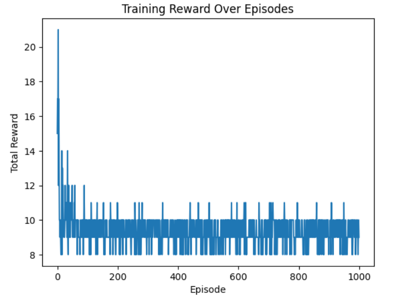
Output graph

Output explanation:

The graph shows the total reward per episode for a reinforcement learning agent across 1,000 episodes. The reward starts high but decreases and stabilizes, indicating the agent may not be improving over time.

Conclusion

This article explored using PyTorch for reinforcement learning, demonstrated through a practical example on the CartPole environment. Starting with simple interactions, the agent learned complex behaviors, such as balancing a pole, through trial and error, guided by rewards. The key takeaway is the power of reinforcement learning to solve problems by learning from actions’ outcomes rather than from direct instruction. The journey from initial failures to consistent success in achieving maximum rewards underscores the learning process’s dynamic and adaptive nature, highlighting reinforcement learning’s potential across various domains. Through this guide, we’ve seen how PyTorch facilitates building and training models for such tasks, offering an accessible pathway for exploring and applying reinforcement learning techniques.