In the world of Reinforcement Learning (RL), two primary approaches dictate how an agent (like a robot or a software program) learns from its environment: On-policy methods and Off-policy methods. Understanding the difference between these two is crucial for grasping the fundamentals of RL. This tutorial aims to demystify the concepts, providing a solid foundation for understanding the nuances between on-policy and off-policy strategies.
Reinforcement Learning
Reinforcement Learning (RL) is an exciting and rapidly evolving field of artificial intelligence that focuses on how agents (like robots or software programs) should take actions in an environment to maximize a notion of cumulative reward. It is inspired by behavioural psychology and revolves around the idea of agents learning optimal behaviour through trial-and-error interactions with their environment. At its core, RL involves an agent, a set of states representing the environment, a set of actions the agent can take, and rewards that the agent receives for performing actions in specific states. The agent’s goal is to learn a policy – a strategy for choosing actions based on states – that maximizes its total reward over time.
One of the key challenges in RL is balancing exploration and exploitation. Exploration involves trying out different actions to discover their effects, while exploitation involves choosing the best-known action to maximize reward. The agent needs to explore enough to find good strategies, but also exploit what it has learned to gain rewards.
What is Policy In Reinforcement Learning (RL)?
A policy is a strategy or set of rules that an agent follows to make decisions in an environment. It defines the mapping from states of the world to the actions the agent should take. Essentially, a policy guides the agent on what action to choose when it encounters a particular state. Policies can be simple, involving fixed actions for each state, or complex, incorporating calculations and learning mechanisms to determine optimal actions. The goal is to find a policy that maximizes the cumulative reward the agent receives over time. Imagine a chess player with a strategy for when to attack, defend, or sacrifice pieces; that’s the player’s policy. In more technical terms, a policy is a mapping from states of the world to the actions the agent should take.
Exploration vs. Exploitation
In the realm of Reinforcement Learning (RL), the delicate balance between exploration and exploitation is a fundamental challenge that agents face in their quest for optimal decision-making.
- Exploration involves the agent trying out new actions to gather information about their effects, potentially leading to the discovery of more rewarding strategies.
- On the other hand, exploitation entails choosing actions that are deemed to be the best based on current knowledge to maximize immediate rewards.
Striking the right balance is crucial; too much exploration can impede progress, while excessive exploitation may lead to suboptimal long-term outcomes. Achieving an optimal trade-off between exploration and exploitation is a nuanced dance that underpins the effectiveness of RL algorithms.
On-Policy Learning In Reinforcement Learning (RL)
On-policy methods are about learning from what you are currently doing. Imagine you’re trying to teach a robot to navigate a maze. In on-policy learning, the robot learns based on the actions it is currently taking. It’s like learning to cook by trying out different recipes yourself. It refers to learning the value of the policy being used by the agent, including the exploration steps. The policy directs the agent’s actions in every state, including the decision-making process while learning. The agent evaluates the outcomes of its present actions, refining its strategy incrementally. This method, much like mastering a skill through hands-on practice, allows the agent to adapt and improve its decision-making by directly engaging with the environment and learning from its own real-time interactions.
SARSA for On-Policy Learning
A prominent example of an on-policy method is SARSA, which stands for State-Action-Reward-State-Action. In SARSA, the agent learns by updating its policy based on the current action (A), the reward (R) received, and the next state-action pair. The update is based on the observed transition without needing a model of the environment’s dynamics. This approach is like learning on the job, where every step you take informs your next decision. SARSA updates the action-value function based on the current action and the following state and action.
Mathematically, it can be represented as:
![Q(s_t,a_t)\leftarrow Q(s_t,a_t)+\alpha[r+\gamma Q(s_{t+1},a_{t+1})-Q(s_t,a_t)]](https://quicklatex.com/cache3/3d/ql_dd701500c24ebd16454d231ed5cc8e3d_l3.png "Rendered by QuickLaTeX.com")
where,
 represents the action-value function, denoting the expected cumulative future rewards of taking action a in state s.
 is the learning rate, determining the step size for the update.
 is the reward received after taking action at
  in state
  and transitioning to state
  .
. is the discount factor, weighing the importance of future rewards.
 is the Q-value for the next state-action pair.
The SARSA algorithm updates its Q-values based on the observed reward and the estimate of future rewards, promoting the learning of an optimal policy over successive iterations.
On-Policy Learning Implementation
Let’s use the OpenAI Gym library, which provides various environments for testing RL algorithms. We will demonstrate both on-policy (using SARSA) and off-policy (using Q-Learning) methods.
Install necessary Python package
!pip install gym
Step 1: Import necessary packages
Python3
import gym
import numpy as np
import matplotlib.pyplot as plt
|
Step 2: Initialize Environment
Python3
env = gym.make('FrozenLake-v1')
env.reset()
|
Step 3: Initialize Q-table and Setting Hyperparameters
The Q-table is a matrix where rows correspond to states in the environment and columns to possible actions. Initially, it’s filled with zeros.
Learning Process
- The agent learns through episodes. In each episode, it starts in an initial state and continues until a terminal state is reached. During each step:
- The agent selects an action based on the current policy, typically using an epsilon-greedy strategy (a mix of exploration and exploitation).
- After performing the action, the agent observes the reward and the new state.
Python3
Q = np.zeros([env.observation_space.n, env.action_space.n])
alpha = 0.1
gamma = 0.99
epsilon = 0.1
num_episodes = 1000
|
Step 4: On-Policy Method (SARSA) Algorithm Implementation
The epsilon-greedy strategy is employed for exploration, and the Q-values are updated using the SARSA formula which considers the reward received and the estimated value of the next action according to the current policy. The code tracks rewards and steps per episode for analysis.
Policy Improvement: Over time, as the agent explores the environment and receives feedback (rewards), the Q-table (representing the policy) gets refined, ideally converging to an optimal policy.
Python
rewards_sarsa = []
steps_per_episode = []
for i in range(num_episodes):
state = env.reset()
done = False
total_reward = 0
step_count = 0
while not done:
if np.random.rand() < epsilon:
action = env.action_space.sample()
else:
action = np.argmax(Q[state, :])
new_state, reward, done, _ = env.step(action)
new_action = np.argmax(Q[new_state, :])
Q[state, action] += alpha * (reward + gamma * Q[new_state, new_action] - Q[state, action])
state = new_state
total_reward += reward
step_count += 1
rewards_sarsa.append(total_reward)
steps_per_episode.append(step_count)
|
Step 5: Visualization
Python3
plt.figure(figsize=(12, 5))
plt.subplot(1, 2, 1)
plt.plot(rewards_sarsa)
plt.title("Rewards per Episode - SARSA")
plt.xlabel("Episode")
plt.ylabel("Total Reward")
plt.subplot(1, 2, 2)
plt.plot(steps_per_episode)
plt.title("Steps per Episode - SARSA")
plt.xlabel("Episode")
plt.ylabel("Steps")
plt.tight_layout()
plt.show()
print("Training complete with SARSA")
|
Output:
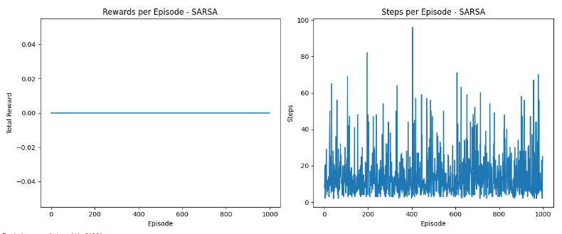
Graphs
- The rewards plot illustrates how the agent’s ability to accumulate rewards evolves over episodes, indicating learning efficiency. A rising trend signifies better strategy formulation.
- The steps plot demonstrates the agent’s efficiency in completing episodes, where a decreasing trend indicates quicker solutions, reflecting improved decision-making over time.
The agent learns based on the current policy it is following, including the exploration steps. It evaluates and improves the policy it uses to make decisions.
Training complete with SARSA
Off-policy learning In Reinforcement Learning (RL)
Off-policy methods, on the other hand, are like learning from someone else’s experience. In this approach, the robot might watch another robot navigate the maze and learn from its actions. It doesn’t have to follow the same policy as the robot it’s observing. It involves learning the value of the optimal policy independently of the agent’s actions. These methods enable the agent to learn from observations about the optimal policy, even when it’s not following it. This is useful for learning from a fixed dataset or a teaching policy.
Importance Sampling
In Reinforcement Learning (RL), importance sampling is a technique used to estimate the expected value of a function under one probability distribution while using samples generated from another distribution. This is particularly relevant in off-policy learning, where an agent learns from a different policy than the one used to generate the data. Importance sampling involves assigning appropriate weights to these samples to correct for the mismatch in distributions, allowing the agent to learn effectively from experiences generated by an external or historical policy. The technique is crucial for improving the efficiency and accuracy of learning algorithms.
Q-Learning for Off-Policy Learning
A classic example of an off-policy method is Q-learning. In Q-learning, our robot would observe the successful moves of other robots and learn the best moves in each state, regardless of what it would do itself in that situation. Think of it as reading a cookbook and learning recipes without actually cooking them yourself. It empowers the agent to distill valuable strategies from external experiences, fostering a versatile and efficient learning paradigm.
Mathematically, it can be represented as:
![Q(s_t, a_t) \leftarrow Q(s_t, a_t) + \alpha \cdot [r_{t+1} + \gamma \cdot \max_a Q(s_{t+1}, a) - Q(s_t, a_t)]](https://quicklatex.com/cache3/60/ql_525c252111dde43ffe762da50aab6060_l3.png "Rendered by QuickLaTeX.com")
Where,
 is the Q-value for state and action .
 is the learning rate (step size).
 is the reward received after taking action in state and transitioning to state .
- is the discount factor.
 is the maximum Q-value over all possible actions in the next state.
On-Policy vs Off-Policy in Reinforcement Learning (RL)
The key difference lies in how these methods approach learning:
- On-policy: Learn from your own current strategy (even if it’s not the best one yet).
- Off-policy: Learn from a different strategy (potentially better or more informed) than what you’re currently using.
- The primary distinction lies in how they approach exploration and exploitation, which affects their convergence properties and practical performance in different types of environments.
Imagine you’re trying to learn how to ride a bike. You try different approaches, fall a few times, and learn from these direct experiences. In RL, this is similar to algorithms that learn from the current policy they are following. The policy is a set of rules or strategies that the algorithm uses to make decisions. In on-policy methods, the algorithm evaluates and improves the policy based on the actions it takes and the outcomes it observes. A well-known example of an on-policy method is the Temporal Difference (TD) learning.
Now, Suppose you’re watching videos of people riding bikes and learning from their experiences, not just your own. In RL, off-policy methods allow the algorithm to learn from a different policy than the one it is currently using. This means the algorithm can learn from past experiences or even from hypothetical situations. This approach is often more flexible and efficient. A popular off-policy method is Q-learning, where the algorithm learns a value function that helps it determine the best action to take in various situations.
In practice, these two approaches have their own advantages and disadvantages:
On-policy methods are straightforward since you’re learning from your own trials and errors. However, they can be less efficient since you might be learning from suboptimal actions.
Off-policy methods, like Q-learning, can be more efficient since you’re learning from potentially optimal actions. But they can be more complex to implement since you’re trying to reconcile what you observe with what you do.
How SARSA and Q-learning works?
On-policy methods like SARSA directly evaluate or improve the policy that the agent follows, while off-policy methods like Q-Learning use data that may be off-policy (i.e., data generated from a different policy) to evaluate or improve the target policy. SARSA takes the next action based on the current policy (which includes exploration), while Q-Learning estimates the return for the best action at the next state (which implicitly assumes a greedy policy).
In-depth, both methods involve iterative processes where the values of states or state-action pairs are updated repeatedly based on experiences (transitions in the case of SARSA and max over next state-action pairs in the case of Q-Learning). Over time, these updates lead to the convergence of the values toward the true values prescribed by the optimal policy.
Off-Policy Method (Q-Learning) Example:
All the first steps will remain same.
Similar to SARSA, the environment is initialized, and a Q-table is created with all entries initially set to zero.
- The agent also learns through episodes. However, the approach to updating the Q-table differs:
- The agent selects an action using the epsilon-greedy strategy.
- Upon taking the action, the agent observes the reward and the new state.
- Unlike SARSA, the Q-table update in Q-Learning is based on the maximum potential value from the next state, regardless of the policy being followed. This reflects the off-policy nature of the algorithm.
- The Q-table update rule in Q-Learning aims to estimate the optimal policy, even if the agent’s current actions are suboptimal or exploratory.
- Over numerous episodes, the Q-table is expected to converge, providing an estimation of the optimal policy. This happens as the agent continually updates the Q-table based on the maximum expected future rewards.
Python
import gym
import numpy as np
import matplotlib.pyplot as plt
env = gym.make('FrozenLake-v1')
env.reset()
Q = np.zeros([env.observation_space.n, env.action_space.n])
alpha = 0.1
gamma = 0.99
epsilon = 0.1
num_episodes = 1000
rewards_q_learning = []
steps_per_episode_q = []
for i in range(num_episodes):
state = env.reset()
done = False
total_reward = 0
step_count = 0
while not done:
if np.random.rand() < epsilon:
action = env.action_space.sample()
else:
action = np.argmax(Q[state, :])
new_state, reward, done, _ = env.step(action)
Q[state, action] += alpha * (reward + gamma * np.max(Q[new_state, :]) - Q[state, action])
state = new_state
total_reward += reward
step_count += 1
rewards_q_learning.append(total_reward)
steps_per_episode_q.append(step_count)
plt.figure(figsize=(12, 5))
plt.subplot(1, 2, 1)
plt.plot(rewards_q_learning)
plt.title("Rewards per Episode - Q-Learning")
plt.xlabel("Episode")
plt.ylabel("Total Reward")
plt.subplot(1, 2, 2)
plt.plot(steps_per_episode_q)
plt.title("Steps per Episode - Q-Learning")
plt.xlabel("Episode")
plt.ylabel("Steps")
plt.tight_layout()
plt.show()
print("Training complete with Q-Learning")
|
Output:
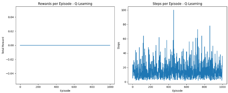
Graphs
Training complete with Q-Learning
In Q-Learning, the visualization also includes rewards and steps per episode. The rewards plot is crucial for observing the agent’s progress in maximizing rewards, where an upward trajectory implies more effective learning of the optimal policy. The steps plot reveals the agent’s efficiency in navigating the environment, with fewer steps per episode indicating more direct paths to the goal, showcasing the algorithm’s efficiency in learning the optimal route.
The agent learns from a policy different from the one it uses to make decisions. It can learn from an optimal or pre-determined policy, regardless of its current strategy.
Conclusion
In conclusion, the distinction between on-policy and off-policy reinforcement learning methods, such as SARSA and Q-learning, is pivotal in tailoring learning strategies to specific task requirements. On-policy methods excel in ensuring safety and continuous adaptation by learning directly from their own experiences. Conversely, off-policy methods, like Q-learning, leverage a broader range of experiences, proving advantageous in environments where discovering optimal solutions outweighs potential risks. The informed choice between these strategies enhances the efficacy of reinforcement learning applications, facilitating more adaptive and efficient learning models across diverse scenarios.
Share your thoughts in the comments
Please Login to comment...