Backpropagation in Machine Learning

Machine learning models learn from data and make predictions. One of the fundamental concepts behind training these models is backpropagation. In this article, we will explore what backpropagation is, why it is crucial in machine learning, and how it works.

A neural network is a network structure, by the presence of computing units(neurons) the neural network has gained the ability to compute the function. The neurons are connected with the help of edges, and it is said to have an assigned activation function and also contains the adjustable parameters. These adjustable parameters help the neural network to determine the function that needs to be computed by the network. In terms of activation function in neural networks, the higher the activation value is the greater the activation is.

What is backpropagation?

• In machine learning, backpropagation is an effective algorithm used to train artificial neural networks, especially in feed-forward neural networks.
• Backpropagation is an iterative algorithm, that helps to minimize the cost function by determining which weights and biases should be adjusted. During every epoch, the model learns by adapting the weights and biases to minimize the loss by moving down toward the gradient of the error. Thus, it involves the two most popular optimization algorithms, such as gradient descent or stochastic gradient descent.
• Computing the gradient in the backpropagation algorithm helps to minimize the cost function and it can be implemented by using the mathematical rule called chain rule from calculus to navigate through complex layers of the neural network.

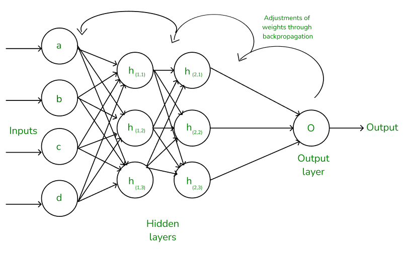
fig(a) A simple illustration of how the backpropagation works by adjustments of weights

Advantages of Using the Backpropagation Algorithm in Neural Networks

Backpropagation, a fundamental algorithm in training neural networks, offers several advantages that make it a preferred choice for many machine learning tasks. Here, we discuss some key advantages of using the backpropagation algorithm:

1. Ease of Implementation: Backpropagation does not require prior knowledge of neural networks, making it accessible to beginners. Its straightforward nature simplifies the programming process, as it primarily involves adjusting weights based on error derivatives.
2. Simplicity and Flexibility: The algorithm’s simplicity allows it to be applied to a wide range of problems and network architectures. Its flexibility makes it suitable for various scenarios, from simple feedforward networks to complex recurrent or convolutional neural networks.
3. Efficiency: Backpropagation accelerates the learning process by directly updating weights based on the calculated error derivatives. This efficiency is particularly advantageous in training deep neural networks, where learning features of a function can be time-consuming.
4. Generalization: Backpropagation enables neural networks to generalize well to unseen data by iteratively adjusting weights during training. This generalization ability is crucial for developing models that can make accurate predictions on new, unseen examples.
5. Scalability: Backpropagation scales well with the size of the dataset and the complexity of the network. This scalability makes it suitable for large-scale machine learning tasks, where training data and network size are significant factors.

In conclusion, the backpropagation algorithm offers several advantages that contribute to its widespread use in training neural networks. Its ease of implementation, simplicity, efficiency, generalization ability, and scalability make it a valuable tool for developing and training neural network models for various machine learning applications.

Working of Backpropagation Algorithm

The Backpropagation algorithm works by two different passes, they are:

• Forward pass
• Backward pass

How does Forward pass work?

• In forward pass, initially the input is fed into the input layer. Since the inputs are raw data, they can be used for training our neural network.
• The inputs and their corresponding weights are passed to the hidden layer. The hidden layer performs the computation on the data it receives. If there are two hidden layers in the neural network, for instance, consider the illustration fig(a), h₁ and h₂ are the two hidden layers, and the output of h₁ can be used as an input of h₂. Before applying it to the activation function, the bias is added.
• To the weighted sum of inputs, the activation function is applied in the hidden layer to each of its neurons. One such activation function that is commonly used is ReLU can also be used, which is responsible for returning the input if it is positive otherwise it returns zero. By doing this so, it introduces the non-linearity to our model, which enables the network to learn the complex relationships in the data. And finally, the weighted outputs from the last hidden layer are fed into the output to compute the final prediction, this layer can also use the activation function called the softmax function which is responsible for converting the weighted outputs into probabilities for each class.
  

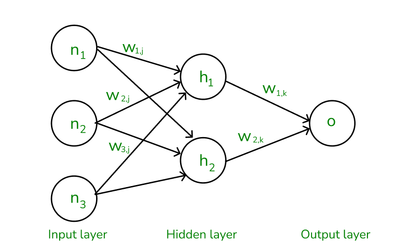
The forward pass using weights and biases

How does backward pass work?

• In the backward pass process shows, the error is transmitted back to the network which helps the network, to improve its performance by learning and adjusting the internal weights.
• To find the error generated through the process of forward pass, we can use one of the most commonly used methods called mean squared error which calculates the difference between the predicted output and desired output. The formula for mean squared error is: [Tex]Mean squared error = (predicted output – actual output)^2 [/Tex]

• Once we have done the calculation at the output layer, we then propagate the error backward through the network, layer by layer.
• The key calculation during the backward pass is determining the gradients for each weight and bias in the network. This gradient is responsible for telling us how much each weight/bias should be adjusted to minimize the error in the next forward pass. The chain rule is used iteratively to calculate this gradient efficiently.
• In addition to gradient calculation, the activation function also plays a crucial role in backpropagation, it works by calculating the gradients with the help of the derivative of the activation function.

Example of Backpropagation in Machine Learning

Let us now take an example to explain backpropagation in Machine Learning,

Assume that the neurons have the sigmoid activation function to perform forward and backward pass on the network. And also assume that the actual output of y is 0.5 and the learning rate is 1. Now perform the backpropagation using backpropagation algorithm.

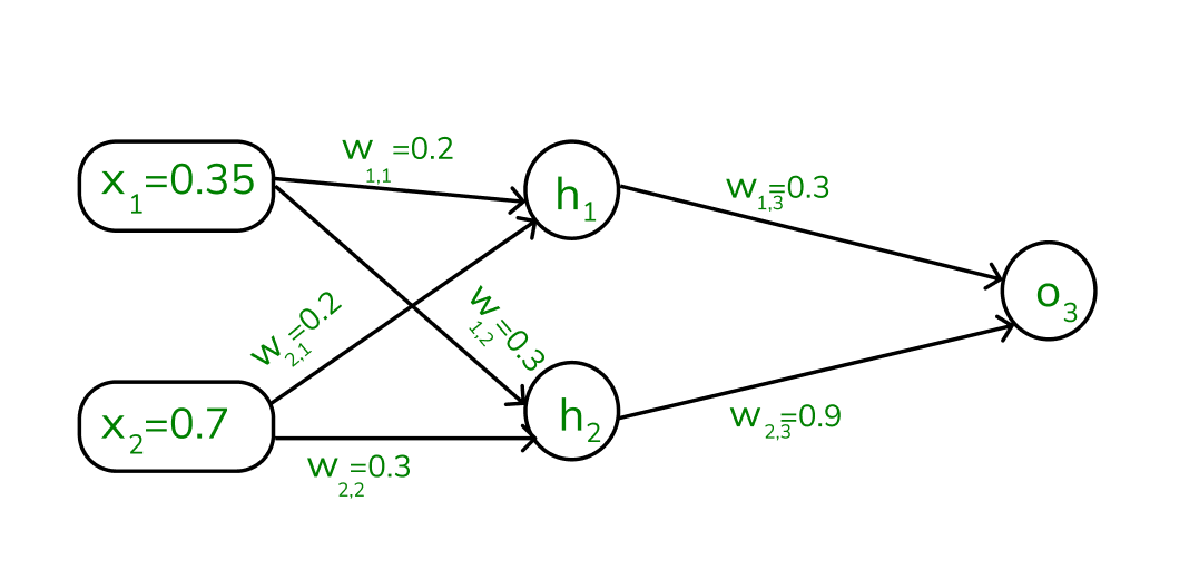
Example (1) of backpropagation sum

Implementing forward propagation:

Step1: Before proceeding to calculating forward propagation, we need to know the two formulae:

[Tex]a_j = \sum (w_i,j * x_i) [/Tex]

Where,

• a_j is the weighted sum of all the inputs and weights at each node,
• wi,j – represents the weights associated with the j^th input to the i^th neuron,
• x_i – represents the value of the j^th input,

[Tex]y_j = F(a_j) = \frac 1 {1+e^{-aj}}[/Tex], y_i – is the output value, F denotes the activation function [sigmoid activation function is used here), which transforms the weighted sum into the output value.

Step 2: To compute the forward pass, we need to compute the output for y₃ , y₄ , and y₅.

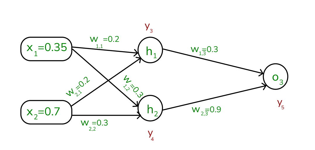
To find the outputs of y3, y4 and y5

We start by calculating the weights and inputs by using the formula:

[Tex]a_j = ∑ (w_{i,j} * x_i) [/Tex] To find y₃ , we need to consider its incoming edges along with its weight and input. Here the incoming edges are from X₁ and X₂.

At h1 node,

[Tex]\begin {aligned} a_1 &= (w_{1,1} x_1) + (w_{2,1} x_2) \\& = (0.2 * 0.35) + (0.3* 0.7) \\&= 0.28 \end {aligned}[/Tex]

Once, we calculated the a₁ value, we can now proceed to find the y₃ value:

[Tex]y_j= F(a_j) = \frac 1 {1+e^{-aj}}[/Tex]

[Tex]y_3 = F(0.28) = \frac 1 {1+e^{-0.28}}[/Tex]

[Tex]y_3 = 0.57[/Tex]

Similarly find the values of y₄ at h₂ and y₅ at O_{3 ,}

[Tex]a2 = (w_{1,2} * x_1) + (w_{2,2} * x_2) = (0.3*0.35)+(0.3*0.7)=0.315[/Tex]

[Tex]y_4 = F(0.315) = \frac 1{1+e^{-0.315}}[/Tex]

[Tex]a3 = (w_{1,3}*y_3)+(w_{2,3}*y_4) =(0.3*0.57)+(0.9*0.59) =0.702[/Tex]

[Tex]y_5 = F(0.702) = \frac 1 {1+e^{-0.702} } = 0.67 [/Tex]

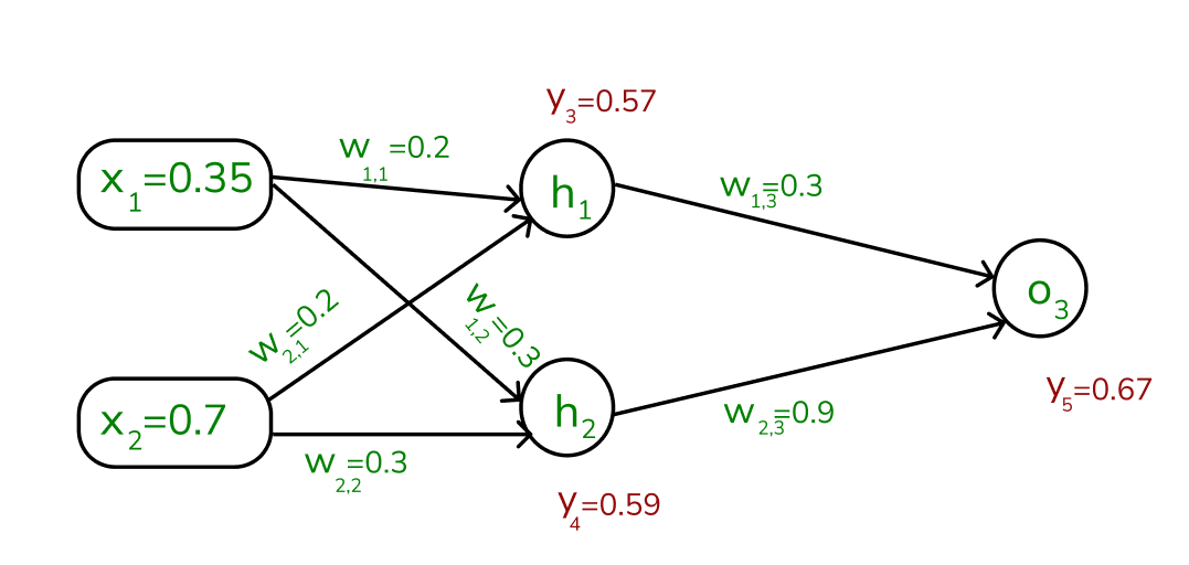
Values of y3, y4 and y5

Note that, our actual output is 0.5 but we obtained 0.67. To calculate the error, we can use the below formula:

[Tex]Error_j= y_{target} – y_5[/Tex]

Error = 0.5 – 0.67

= -0.17

Using this error value, we will be backpropagating.

Implementing Backward Propagation

Each weight in the network is changed by,

∇wij = η 𝛿j Oj 𝛿j = Oj (1-Oj)(tj - Oj) (if j is an output unit) 𝛿j = Oj (1-O)∑k 𝛿k wkj (if j is a hidden unit) where ,

η is the constant which is considered as learning rate,

t_j is the correct output for unit j

𝛿_j is the error measure for unit j

Step 3: To calculate the backpropagation, we need to start from the output unit:

To compute the 𝛿₅, we need to use the output of forward pass,

𝛿₅ = y₅(1-y₅) (y_target -y₅)

= 0.67(1-0.67) (-0.17)

= -0.0376

For hidden unit,

To compute the hidden unit, we will take the value of 𝛿₅

𝛿₃ = y₃(1-y₃) (w_1,3 * 𝛿₅)

=0.57(1-0.57) (0.3*-0.0375)

=-0.0027

𝛿₄ = y₄ (1-y₅) (w_2,3 * 𝛿₅)

=0.59(1-0.59) (0.9*-0.376)

=-0.0819

Step 4: We need to update the weights, from output unit to hidden unit,

∇ wj,i = η 𝛿j Oj

Note- Here our learning rate is 1

∇ w_2,3 = η 𝛿₅ O₄

= 1 * (-0.376) * 0.59

= -0.22184

We will be updating the weights based on the old weight of the network,

w_2,3(new) = ∇ w_4,5 + w_4,5 (old)

= -0.22184 + 0.9

= 0.67816

From hidden unit to input unit,

For an hidden to input node, we need to do calculations by the following;

∇ w_1,1 = η 𝛿₃ O₄

= 1 * (-0.0027) * 0.35

= 0.000945

Similarly, we need to calculate the new weight value using the old one:

w_1,1(new) = ∇ w_1,1+ w_1,1 (old)

= 0.000945 + 0.2

= 0.200945

Similarly, we update the weights of the other neurons: The new weights are mentioned below

w_1,2 (new) = 0.271335

w_1,3 (new) = 0.08567

w_2,1 (new) = 0.29811

w_2,2 (new) = 0.24267

The updated weights are illustrated below,

Through backward pass the weights are updated

Once, the above process is done, we again perform the forward pass to find if we obtain the actual output as 0.5.

While performing the forward pass again, we obtain the following values:

y₃ = 0.57

y₄ = 0.56

y₅ = 0.61

We can clearly see that our y₅ value is 0.61 which is not an expected actual output, So again we need to find the error and backpropagate through the network by updating the weights until the actual output is obtained.

[Tex]Error = y_{target} – y_5[/Tex]

= 0.5 – 0.61

= -0.11

This is how the backpropagate works, it will be performing the forward pass first to see if we obtain the actual output, if not we will be finding the error rate and then backpropagating backwards through the layers in the network by adjusting the weights according to the error rate. This process is said to be continued until the actual output is gained by the neural network.

Python program for backpropagation

Here’s a simple implementation of feedforward neural network with backpropagation in Python:

1. Neural Network Initialization: The NeuralNetwork class is initialized with parameters for the input size, hidden layer size, and output size. It also initializes the weights and biases with random values.
2. Sigmoid Activation Function: The sigmoid method implements the sigmoid activation function, which squashes the input to a value between 0 and 1.
3. Sigmoid Derivative: The sigmoid_derivative method calculates the derivative of the sigmoid function. It computes the gradients of the loss function with respect to weights.
4. Feedforward Pass: The feedforward method calculates the activations of the hidden and output layers based on the input data and current weights and biases. It uses matrix multiplication to propagate the inputs through the network.
5. Backpropagation: The backward method performs the backpropagation algorithm. It calculates the error at the output layer and propagates it back through the network to update the weights and biases using gradient descent.
6. Training the Neural Network: The train method trains the neural network using the specified number of epochs and learning rate. It iterates through the training data, performs the feedforward and backward passes, and updates the weights and biases accordingly.
7. XOR Dataset: The XOR dataset (X) is defined, which contains input pairs that represent the XOR operation, where the output is 1 if exactly one of the inputs is 1, and 0 otherwise.
8. Testing the Trained Model: After training, the neural network is tested on the XOR dataset (X) to see how well it has learned the XOR function. The predicted outputs are printed to the console, showing the neural network’s predictions for each input pair.

Python

import numpy as np

class NeuralNetwork:
    def __init__(self, input_size, hidden_size, output_size):
        self.input_size = input_size
        self.hidden_size = hidden_size
        self.output_size = output_size

        # Initialize weights
        self.weights_input_hidden = np.random.randn(self.input_size, self.hidden_size)
        self.weights_hidden_output = np.random.randn(self.hidden_size, self.output_size)

        # Initialize the biases
        self.bias_hidden = np.zeros((1, self.hidden_size))
        self.bias_output = np.zeros((1, self.output_size))

    def sigmoid(self, x):
        return 1 / (1 + np.exp(-x))

    def sigmoid_derivative(self, x):
        return x * (1 - x)

    def feedforward(self, X):
        # Input to hidden
        self.hidden_activation = np.dot(X, self.weights_input_hidden) + self.bias_hidden
        self.hidden_output = self.sigmoid(self.hidden_activation)

        # Hidden to output
        self.output_activation = np.dot(self.hidden_output, self.weights_hidden_output) + self.bias_output
        self.predicted_output = self.sigmoid(self.output_activation)

        return self.predicted_output

    def backward(self, X, y, learning_rate):
        # Compute the output layer error
        output_error = y - self.predicted_output
        output_delta = output_error * self.sigmoid_derivative(self.predicted_output)

        # Compute the hidden layer error
        hidden_error = np.dot(output_delta, self.weights_hidden_output.T)
        hidden_delta = hidden_error * self.sigmoid_derivative(self.hidden_output)

        # Update weights and biases
        self.weights_hidden_output += np.dot(self.hidden_output.T, output_delta) * learning_rate
        self.bias_output += np.sum(output_delta, axis=0, keepdims=True) * learning_rate
        self.weights_input_hidden += np.dot(X.T, hidden_delta) * learning_rate
        self.bias_hidden += np.sum(hidden_delta, axis=0, keepdims=True) * learning_rate

    def train(self, X, y, epochs, learning_rate):
        for epoch in range(epochs):
            output = self.feedforward(X)
            self.backward(X, y, learning_rate)
            if epoch % 4000 == 0:
                loss = np.mean(np.square(y - output))
                print(f"Epoch {epoch}, Loss:{loss}")

X = np.array([[0, 0], [0, 1], [1, 0], [1, 1]])
y = np.array([[0], [1], [1], [0]])

nn = NeuralNetwork(input_size=2, hidden_size=4, output_size=1)
nn.train(X, y, epochs=10000, learning_rate=0.1)

# Test the trained model
output = nn.feedforward(X)
print("Predictions after training:")
print(output)

Output:

Epoch 0, Loss:0.36270360966344145 Epoch 4000, Loss:0.005546947165311874 Epoch 8000, Loss:0.00202378766386817 Predictions after training: [[0.02477654] [0.95625286] [0.96418129] [0.04729297]]