Model-Free Reinforcement Learning: An Overview

In Reinforcement learning, we have agents that use a particular ‘algorithm’ to interact with the environment.

Now this algorithm can be model-based or model-free.

• The traditional algorithms are model-based in the sense they tend to develop a ‘model’ for the environment. This developed model captured the ‘transition probability’ and ‘rewards’ for each state and action that the agent used for planning its action.
• The new age algorithms are model-free in the sense they do not develop a model for the environment. Instead, they develop a policy that guides the agent to take the best possible action in a given state without needing transition probabilities. In the model-free algorithm, the agent learns by hit and trial method by interacting with the environment.

In this article we will first get a basic overview of RL, then we will discuss the difference between model-based and model-free algorithms in detail. Then we will study the Bellman equation which is the basis of the model-free learning algorithm and then we will see the difference between on-policy and off-policy, value-based, and policy-based model-free algorithms. Then we will get an overview of major model-free algorithms. Finally, we will do a simple implementation of the Q-learning algorithm using an open AI gym.

Reinforcement Learning

Generally, when we talk about machine learning problems, we think of categorizing them into supervised and unsupervised learning. However, there is another less glamorized category which is reinforcement learning (RL).

In reinforcement learning, we train an agent by making it interact with the environment. Unlike supervised learning or unsupervised learning where we have an unlabeled or labeled dataset to start with, in reinforcement learning there is no data to start with. The agent gets the data from its interaction with the environment. It uses this data to either build an optimal policy that could guide it or build a model that could simulate the environment. In reinforcement learning the objective of the agent is to learn a policy /model that would decide the behavior of the agent in an environment

Here by environment, we mean a dynamic context in which the agent operates. For example, think of a self-driving car. The road, the signal, the pedestrian, another vehicle, etc. is the environment. The self-driving car (‘agent’) interacts with the ‘environment’ through ‘action’ (moving, accelerating turning right/left, stopping, etc.). For each interaction, the environment produces a new state and ‘reward’ (notional high value for correct moves, notional low values for incorrect values). Through these rewards, the agent learns a ‘policy’ or ‘model’. The ‘policy’ or ‘model’ describes what action needs to be taken by the agent in a given ‘state’.

All the above components described are the components of the Markov Decision Process (MDP). Formally MDP consists of

• Agent: A reinforcement learning agent is the entity that we are training to make correct decisions.
• Environment: The environment is the surroundings with which the agent interacts.
• State: The state defines the current situation of the agent
• Action: The choice that the agent makes at the current time step.
• Policy/Model: A policy guides the agent to take action.
• Reward: The positive or negative outcome of the interaction of the agent with the environment

Model-based vs Model Free Reinforcement Learning (RL)

The environment with which the agent interacts is a black box for the agent i.e. how it operates is not known to the agent. Based on what the agent tries to learn about this black box we can define the RL in two categories.

Model-Based

• In model-based RL the agent tries to understand how the environment is generating outcomes and rewards. The idea is to understand how the environment produces the outcomes that it produces to develop a ‘model’ that can simulate the environment.
• This model is used to simulate possible future state s’ and outcomes, allowing the agent to plan and make decisions based on these simulations.
• Here the agent can estimate the reward of the action beforehand without interacting with the environment as it now has a model or a simulator that behaves like the environment.
• Ultimately the model learns the transition probability (probability of going from one state to another state and then to another state) and which transition produces good rewards.
• For example, consider an agent interacting with a computer chess. Here the agent can try to learn that if I move a particular piece on the chess board what could be the response of my opponent. Based on its interaction, the agent will try to build a model that would have learned all the strategies and nuances of playing a game of chess from start to finish.
• Example Dynamic Programming Policy Evaluation

Model-free

• Here the RL agent does not try to understand the environment dynamics. Instead, it builds a guide (policy) for itself that tells what the optimal behavior in a is given state i.e. the best action to be taken in a given state. This is built using error and trial methods by the agent.
• Here the agent cannot predict or guess what will be future output of its action. It well known to the agent only in real-time.
• In model-free RL, the focus is on learning by observing the consequences of actions rather than attempting to understand the dynamics of the environment.
• The agent does not estimate the transition probability distribution (and the reward function) associated with the environment.
• This approach is particularly useful in situations where the underlying model is either unknown or too complex to be accurately represented.
• For example, consider the game of cards – We have a handful of cards in our hand, and we must pick one card to play. Here instead of thinking of all possible future outcomes associated with playing each card which is nearly impossible to model the agent will try to learn what is the best card to play given the current hands of the card based on its interaction with the environment.
• Examples of such algorithms are SARSA, Policy Gradient, Q-learning, Deep Q
• It is important to note that most of the focus now is on the Model-free RL and it is what most people mean when they say the term ‘Reinforcement Learning.

So, in the remainder of this article, we will be focusing our discussion on only Model free approaches of RL. Model-free algorithms are generally further characterized by whether there are value-based, or policy based and on-policy or off-policy.

Value-based and Policy Based RL

• Value Based: Here we don’t store any policy. Instead, policy is derived from value function. Value-based RL builds a Q value function for state action pairs. These Q values quantify the expected reward of taking a particulate action in a given state. The policy is derived from this function which is generally the action with the best Q value.
• Policy Based: In the policy-based method we don’t build a function for state value. Instead, the method focuses on making a policy for state value pairs which is the probability of taking a particular action in a given state that maximizes the reward. This probability could either be stochastic or determinist.

Off Policy and On Policy Model Free RL

This division is generally done for value-based policy on how the Q values are updated.

• Off Policy: In this behavioral policy i.e. the policy with which it picks up the action and the policy that it is to learn is different. Suppose you are in state s and make an action that leads you to state s’. If we update our Q function on the best possible action in s’ then we have off-policy RL. This will become clearer when we discuss the Q learning algorithm below.
• On Policy: In this the behavioral policy and target policy are the same. Suppose you are in state s and make an action that leads you to state s’. If we update our Q function on the action taken in states’ then we have on policy RL

Bellman Equation in RL

The Bellman equation is the foundation of many algorithms in RL. It has many forms depending on the type of algorithm and the value being optimized.

The return for any state action value is decomposed into two parts.

• Immediate reward from the action that is taken to reach the next stage.
• The Discounted return from that next state by following the same policy for all subsequent steps.

This recursive relationship is known as the Bellman Equation.

V(S₁) = E[R + YV(S₂)]

Let us understand Bellman equation with the help of the q value.

For example, Bellman considers the q value in valued based model free RL. When we build a value function in an RL algorithm, we update it with a value called Q i.e. Quality value for each state action pair.

Consider a simple naive environment where there are only 5 possible state s’ and 4 possible actions. Hence, we can develop a look-up table with rows representing the state s’ and columns representing the value. Each of the values in the matrix represents the reward obtained by taking that particle action given the agent is in that state. This value is known as the q value. It is this q value that the agent learns through its interaction with the environment. Once the agent has interacted with the environment for a sufficient amount of time the value contained in the table will be optimal values. Based on this value the agent will decide its action.

Formally the Q-value of a state-action pair is denoted as Q(s, a), where:

• s is the current state of the environment.
• a is the action taken by the agent.

Bellman equation expresses the relationship between the value of a state (or state-action pair) and the expected future rewards achievable from that state.

Whenever an agent interacts with an environment it gets two things in return – the immediate reward for that action and its successor state. Based on these two it updates the Q value of the current state

Q(s,a) = E [R_t+1 + max(Q(s’,a’)]

The expected return from starting state s, taking action a, and with the optimal policy afterward will be equal to the expected reward R_t+1 we can get by selecting action a in state s plus the maximum of “expected discounted return” that is achievable of any (s′, a′) where (s′, a′) is a potential next state-action pair

Model-Free Algorithms

Let us discuss some popular model-free algorithms.

Q-learning

Q-learning is a classic RL algorithm that aims to learn the quality of actions in a given state. The Q-value represents the expected cumulative reward of taking a particular action in a specific state. We covered the Q learning algorithm in detail when we discussed the on-policy model-free algorithm.

In this behavioral policy i.e. the policy with which it picks up the action and the policy that it is to learn is different. The bellman equation is given by:

• s – current state of the environment.
• a – is the action taken by the agent.
• α – is a learning rate a number that controls the size of the updates of the Q-values.
• r – is the reward received by the agent for taking action in state s
• β – is a discount factor that decides what importance must be given to immediate rewards concerning future rewards when making a decision.
• s’, a’ – are new state s and actions in the new state.

SARSA

SARSA stands for State Action Reward State Action. The updated equation for SARSA depends on the current state, current action, reward obtained, next state, and next action. SARSA operates by choosing an action following the current epsilon-greedy policy and updates its Q-values accordingly.

In this, the behavioral policy and target policy is the same. The Bellman equation for state action value pair is given by:

• Note the difference w.r.t to Q value. Here instead of updating with the maximum q value of the future state, we update the Q value associated with the actual action that the agent has taken in the next state.
• Here the behavior-making policy and update to the target policy are the same. Whatever the behavior chosen by the agent, the update to the q value is done according to the q value associated with it.
• The agent evaluates and updates its policy based on the data it collects while following that policy.
• The data used for learning comes from the same policy that is being improved.
• This type of policy is followed when there is a cost associated with a wrong action.
  • Training a robot on walking downstairs. If it places a wrong foot, there will be costs associated with physical damage.

DQN

DQN is based on the Q learning algorithm. It integrates the deep learning technique with Q learning. In Q learning we develop a table for state action pairs. However, this is not feasible in scenarios where the number of state action pairs reaches high. So instead of making a value function like a table we develop a neural network that plays the role of a function that outputs quality value for a given input of state and action. So instead of using a table to store Q-values for each state-action pair, a deep neural network is used to approximate the Q-function.

Actor Critic

Actor critic combines elements of both policy-based (actor) and value-based (critic) methods. The main idea is to have two components working together: an actor, which learns a policy to select actions, and a critic, which evaluates the chosen actions.

• The actor is responsible for selecting actions based on the current policy which is policy-based based.
• The critic evaluates the actions taken by the actor by estimating the value or advantage function which is value-based.

Implementation of Model Free RL

We will use OpenAI gymnasium (also known formerly as OpenAI gym) to build a model-free RL using a Q learning algorithm (off policy). Now to train an RL agent we need an environment that can provide a simulation of the environment. This is what the open gym toolkit does. It provides a variety of environments that can be used for testing different reinforcement learning algorithms. Users can also create and register their custom environments in OpenAI Gym, allowing them to test algorithms on specific tasks relevant to their research or application.

Just as Pytorch or TensorFlow have become the standard framework for implementing deep learning tasks, OpenAI gym has become the default standard for benchmarking and evaluation of RL algorithms.

To install the gymnasium, we can use the below command

!pip install gymnasium

1. Understand the environment

We will be using the taxi-v3 environment from the OpenAI gym.

• The OpenAI Gym Taxi-v3 environment is a classic reinforcement learning problem often used for learning and testing RL algorithms. In this environment, the agent controls a taxi navigating a grid world, to pick up a passenger from one location and drop them off at another.
• The setting consists of a 5 * 5 gird.
• The taxi driver is shown with a yellow background.
• There are walls represented by vertical lines.
• The goal is to move the taxi to the passenger’s location (colored in blue), pick up the passenger, move to the passenger’s desired destination (colored in purple), and drop off the passenger.
• The agent is rewarded as follows:
  • +20 for successfully dropping off the passenger.
  • -10 for unsuccessful attempts to pick up or drop off the passenger.
  • -1 for each step taken by the agent, aiming to encourage the agent to take an efficient route.

Python3

import gymnasium as gym
env = gym.make('Taxi-v3',render_mode='ansi')
env.reset()

print(env.render())

Output:

Taxi-V3 environment

• The gym.make(‘Taxi-v3′, render_mode=’ansi’) line creates an instance of the Taxi-v3 environment. The render_mode=’ansi’ argument specifies the rendering mode to be in ANSI mode, which is a text-based mode suitable for displaying the environment in a text console
• The env.reset() method is called to reset the environment to its initial state. This is typically done at the beginning of each episode to start fresh.

2. Create the q learning agent

• Initialization (__init__ method):
  • env: The environment in which the agent operates.
  • learning_rate: The learning rate for updating Q-values.
  • initial_epsilon: The initial exploration rate.
  • epsilon_decay: The rate at which the exploration rate decreases.
  • final_epsilon: The minimum exploration rate.
  • discount_factor: The discount factor for future rewards.
• get_action method:
  • With probability ε, it chooses a random action (exploration).
  • With probability 1-ε it chooses the action with the highest Q-value for the current observation (exploitation).
  • This value is high initially and gradually reduced
• update method:
  • Updates the Q-value based on the observed reward and the maximum Q-value of the next state.
• decay_epsilon method:
  • decreases the exploration rate (epsilon) until it reaches its final value.

Python3

import numpy as np
from collections import defaultdict
import matplotlib.pyplot as plt


class QLearningAgent:
    def __init__(self, env, learning_rate, initial_epsilon, epsilon_decay, final_epsilon, discount_factor=0.95
                 ):
        self.env = env
        self.learning_rate = learning_rate
        self.discount_factor = discount_factor

        self.epsilon = initial_epsilon
        self.epsilon_decay = epsilon_decay
        self.final_epsilon = final_epsilon

        # Initialize an empty dictionary of state-action values
        self.q_values = defaultdict(lambda: np.zeros(env.action_space.n))

    def get_action(self, obs) -> int:
        x = np.random.rand()
        if x < self.final_epsilon:
            return self.env.action_space.sample()
        else:
            return np.argmax(self.q_values[obs])

    def update(self, obs, action, reward, terminated, next_obs):
        if not terminated:
            future_q_value = np.max(self.q_values[next_obs])
            self.q_values[obs][action] += self.learning_rate * \
                (reward + self.discount_factor *
                 future_q_value-self.q_values[obs][action])

    def decay_epsilon(self):
        """Decrease the exploration rate epsilon until it reaches its final value"""
        self.epsilon = max(self.final_epsilon,
                           self.epsilon - self.epsilon_decay)

3. Define our training method

• The train_agent function is responsible for training the provided Q-learning agent in a given environment over a specified number of episodes.
• Each episode is one iteration either till the agent makes a mistake leading to termination or completes drop-off successfully.
• The function iterates through the specified number of episodes (episodes).
• Episode Initialization:
  • It resets the environment and initializes variables to track episode progress.
• Within each episode, the agent
  • Selects actions based on the method defined in our agent class,
  • Interacts with the environment,
  • updates Q-values and accumulates rewards until the episode terminates.
• Epsilon Decay:
  • After each episode, the agent’s exploration rate (epsilon) is decayed using the decay_epsilon method.
  • Initially, the epsilon value is high leading to more exploration.
  • This is brought down to 0.1 in half the number of episodes.
• Performance Tracking:
  • The total reward for each episode is stored in the rewards list.
  • We calculate the average of the last 10 episodes and save the best average reward obtained at each episode’s end.
• Print Progress:
  • We print the best average progress at every 100 evaluation intervals,
  • We also return all the rewards that we obtained in each episode. This will help us in plotting.

Python3

def train_agent(agent, env, episodes, eval_interval=100):
    rewards = []
    best_reward = -np.inf
    for i in range(episodes):
        obs, _ = env.reset()
        terminated = False
        truncated = False
        length = 0
        total_reward = 0

        while (terminated == False) and (truncated == False):

            action = agent.get_action(obs)
            next_obs, reward, terminated, truncated, _ = env.step(action)

            agent.update(obs, action, reward, terminated, next_obs)
            obs = next_obs
            length = length+1
            total_reward += reward

        agent.decay_epsilon()
        rewards.append(total_reward)

        if i >= eval_interval:
            avg_return = np.mean(rewards[i-eval_interval: i])
            best_reward = max(avg_return, best_reward)
        if i % eval_interval == 0 and i > 0:

            print(f"Episode{i} -> best_reward={best_reward} ")
    return rewards

4. Running our training method

• Sets up parameters for training, such as the number of episodes, learning rate, discount factor, and exploration rates.
• Creates the Taxi-v3 environment from OpenAI Gym.
• Initializes a Q-learning agent (QLearningAgent) with the specified parameters.
• Calls the train_agent function to train the agent using the specified environment and parameters.

Python3

episodes = 20000
learning_rate = 0.5
discount_factor = 0.95
initial_epsilon = 1
final_epsilon = 0
epsilon_decay = ((final_epsilon-initial_epsilon) / (episodes/2))
env = gym.make('Taxi-v3', render_mode='ansi')
agent = QLearningAgent(env, learning_rate, initial_epsilon,
                       epsilon_decay, final_epsilon)

returns = train_agent(agent, env, episodes)

Output:

Episode100 -> best_reward=-224.3 
Episode200 -> best_reward=-116.22 
Episode300 -> best_reward=-40.75 
Episode400 -> best_reward=-14.89 
Episode500 -> best_reward=-3.9 
Episode600 -> best_reward=1.65 
Episode700 -> best_reward=2.13 
Episode800 -> best_reward=2.13 
Episode900 -> best_reward=3.3 
Episode1000 -> best_reward=4.32 
Episode1100 -> best_reward=6.03 
Episode1200 -> best_reward=6.28 
Episode1300 -> best_reward=7.15 
Episode1400 -> best_reward=7.62 
...

5. Plotting our returns

• We can plot all the rewards obtained against the episode
• We see a gradual decrease in reward value fa from large negative value towards zero and ultimately reaching positive value around 8.6.

Python3

def plot_returns(returns):
    plt.plot(np.arange(len(returns)), returns)
    plt.title('Episode returns')
    plt.xlabel('Episode')
    plt.ylabel('Return')
    plt.show()

plot_returns(returns)

Output:

Plot of rewards

6. Running our Agent

The run_agent function is designed to execute our trained agent in the Taxi-v3 environment and displays its interaction

• agent. epsilon = 0: This line sets the exploration rate (epsilon) of the agent to zero, indicating that the agent should exploit its learned policy without further exploration
• The while loop continues until either the episode terminates (terminated == True) or the interaction is truncated (truncated == True)
• action = agent.get_action(obs): The agent selects an action based on its learned policy
• env.render(): Renders the updated state after the agent’s action.
• obs = next_obs: Updates the current state to the next state for the next iteration.

Python3

def run_agent(agent, env):
    agent.epsilon = 0    # No need to keep exploring
    obs, _ = env.reset() # get the current state
    env.render()
    terminated = truncated = False

    while terminated == False and truncated == False   :
        action = agent.get_action(obs)
        next_obs, _, terminated, truncated, _ = env.step(action)
        print(env.render())

        obs = next_obs

env = gym.make('Taxi-v3', render_mode='ansi')
run_agent(agent, env)

Output:

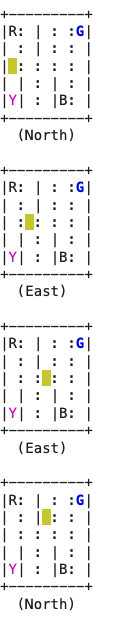
Output of the agent action

Conclusion

In this article, we got an understanding of reinforcement learning, difference between model-free and model-based RL, how q value is determined in model-free RL, the difference between on-policy and off-policy algorithms, and the saw the implementation of the Q learning algorithm.