R Interview Questions

R is a programming language and also a software environment for statistical computing and data analysis. R was developed by Ross Ihaka and Robert Gentleman at the University of Auckland, New Zealand. R is an open-source programming language and it is available on widely used platforms e.g. Windows, Linux and Mac. It generally comes with a command-line interface and provides a vast list of packages for performing tasks. R is an interpreted language that supports both procedural programming and object-oriented programming.

Top 50 R Interview Questions

R is the most used language in top companies such as Facebook, Google, Bing, Accenture, Wipro, and many more. To get into these companies and other software companies, you need to master some important Core R interview questions to crack their R Online Assessment round and R interview. R’s significance in data science stems from its versatility and vast collection of packages, which facilitate various tasks such as data manipulation, visualization, and statistical analysis. Its popularity can be attributed to its active community and the ability to create high-quality, interactive data visualizations.

This article focuses on R programming interview questions and has been written under the guidance of experts in the R programming language. It incorporates valuable insights gathered from recent R interviews with students.

Table of Content

• R Interview Questions for Freshers
• R Interview Questions for Experienced

R Interview Questions for Freshers

1. What is R programming and what are main feature of R?

R Programming Language is an open-source programming language that is widely used as a statistical software and data analysis tool. R generally comes with the Command-line interface. R is available across widely used platforms like Windows, Linux, and macOS. Also, the R programming language is the latest cutting-edge tool.
R programming is used as a leading tool for machine learning, statistics, and data analysis. Objects, functions, and packages can easily be created by R.

The main features of R:

• Open source
• Extensible
• Statistical computing
• Reproducibility
• Graphics

2. What Are Some Advantages and drawbacks of R?

There are some following Advantages and drawbacks of R.

Advantages:

• Open source: R is a programming language that is available for free use, distribution, and modification.
• Large community: R has a sizable and vibrant user and developer base that actively participates in its development and offers support through forums, blogs, and other tools. 
• Numerous packages: R is a highly adaptable and flexible language thanks to the large and expanding number of packages that are available for various data analysis tasks. 
• Statistical computing: R contains a large number of built-in statistical functions and libraries because it was primarily created for statistical computing and analysis. 
• Visualization: R contains strong visualization features that make it possible to create high-quality visualizations, such as charts, plots, and maps.Visualization.

Drawbacks:

• steep learning curve: For people who are unfamiliar with programming or statistical principles, learning R can be challenging. 
• Memory management: R has some memory management issues, which can make it difficult to work with a huge dataset. 
• Limited performance: When it comes to specific tasks like data processing and manipulation, R can be slower than other programming languages like Python or C++. 
• Quality control: Because R is open-source and has a lot of packages, there can be problems with it, and certain packages might not be well-tested or well-documented.

Despite being widely used in academia and research, R may not be as supported in some industries.

3. How to load a .csv file?

To load a .csv file in R, you can use the read.csv() function. Here’s an example:

R

# load the csv file
mydata <- read.csv("filename.csv")

# print the data to check if
# it has loaded correctly
print(mydata)

In this example, we first set the working directory (if it is not already set) to the location where the CSV file is kept. The CSV file is then loaded using the read.csv() function and saved in a variable called my data. In order to ensure that the data has been loaded properly, we print the data at the end using the print() function.

4. Explain with() and by() functions.

• with() function: provides a convenient way to refer to variables within a data frame or environment without explicitly specifying the name of the data frame or environment each time. It allows you to access and manipulate variables within the specified data frame or environment in a more concise manner.
• by() Function: Applying a function or expression to parts of a data frame that have been divided by one or more factors is done using the by() function. On the basis of one or more variables, it enables you to conduct operations on groupings of data.

with() function makes referring variables inside a data frame or environment simpler. The by() function, on the other hand, enables operations on data subsets depending on variables or factors, enabling group-wise analysis or calculations.

5. Explain for loop and while loop in R.

For Loop:

• Repeat a group of sentences or a section of code for a predetermined number of iterations, you use a for loop.
• It is frequently used to loop through a series of values or objects, like a vector or a set of numbers.
• The cycle repeats until each value in the sequence has been handled.

for (variable in sequence) {
                       # Statements or code block to be executed
                                                      }

While Loop:

• Keep repeating a group of statements or a section of code as long as a certain condition holds true, we use a while loop.
• It is frequently used when the number of iterations is unknown in advance or when the loop has to run indefinitely.
• To prevent an infinite loop, it’s crucial to make sure the condition inside the while loop ultimately turns into FALSE.

while (condition) {
              # Statements or code blocks to be executed
                                                         }

6. What is the memory limit of R?

 A 32-bit version of R can only handle a maximum of about 4 GB of memory. This is due to the constrained address space of 32-bit applications.
The memory limit in a 64-bit version of R is substantially greater and is based on the physical memory that is available on the system. Depending on the system configuration, it can be anywhere between a few megabytes and terabytes.

7. How to install and load the package?

To install a package, we can use the install.packages() function. Here’s an example:

install.packages("package_name")

Once a package is installed, we need to load it into our R session to use its functions and features. we can use the library() or require() function to load a package. Here’s an example:

library(package_name)

8. What is a data frame?

A data frame is made up of rows and columns, where each row denotes an observation or record and each column a variable or attribute. A data frame’s columns can include a variety of data kinds, including logical, character, factor, and numeric ones, enabling the storing and management of the data.

9. Explain different data types in R.

Various data types are available in R to represent various types of information. Each data type has unique features, properties, and manipulation functions. Here are a few R data types that are frequently used:

1. Numeric
2. Character
3. Integer
4. Logical
5. Complex

10. How to find missing values in R?

Various functions and methods in R can be used to locate missing values in a data collection or a vector. Here are a few used approaches:

is.na() Function

R

# Creating a vector with missing values
x <- c(1, 2, NA, 4, NA, 6)

# Finding missing values using is.na()
missing_values <- is.na(x)

# Printing the logical vector
print(missing_values)

Output:

[1] FALSE FALSE  TRUE FALSE  TRUE FALSE

complete.cases() Function

R

# Creating a data frame with missing values
df <- data.frame(x = c(1, 2, NA, 4), y = c(NA, "A", "B", "C"))

# Finding complete cases using complete.cases()
complete_cases <- complete.cases(df)

# Printing the logical vector
print(complete_cases)

Output:

[1] FALSE  TRUE FALSE  TRUE

11. What is Rmarkdown? What is the use of it?

R Markdown is a tool that combines the ease of Markdown syntax with the functionality of R programming. It enables us to produce dynamic files that smoothly combine text, code, and output in a single file. Files with the extension have R Markdown. Rmd.

The primary purpose of R Markdown is to facilitate reproducible research and report generation. Here are some key uses and benefits of R Markdown:

1. Reproducibility
2. Mixing Code and Text
3. Integration of Multiple Technologies
4. Collaboration and Sharing
5. Customization and Flexibility
6. Automated Report Generation

12. How to create a user-defined function in R?

Start by defining the function name, input arguments, and the code that will be run when the function is called in order to construct a user-defined function.

The following is the fundamental syntax for defining a function in R:

function_name <- function(arg1, arg2, ...) {
  # Function code
  # Perform calculations or operations
  # Return a value (optional)
}

13. What is the difference between a vector and a list?

In R, a vector and a list are both data structures used to store multiple elements. Here are the key differences between vectors and lists:

Vector	List
A vector is a homogenous data structure. It can only have components that are the same length.	A list is a form of heterogeneous data structure that can contain items of various data types and lengths. It might include matrices, data frames, vectors, or other lists.
A vector is a one-dimensional structure that resembles an array. It can be pictured as a series of components that have been placed in a linear form.	A list is a one-dimensional structure that can accommodate many types of entries. It may be viewed as a group of objects, each of which could be of any size or data type.
Indexing is used to access a vector’s elements. Numerical or logical indexing can be used to access a single element or a collection of elements.	Double square brackets (“[[]]”) or the dollar sign (“$”) are used to access list items. While the dollar sign is used to extract named elements from the list, double square brackets extract a single element.
The length of a vector is determined by the number of elements it contains.	The length of a list is the number of elements it contains, including nested lists.
A vector’s elements can be changed or swapped out using indexing.	Using indexing or assignment, we can change or replace a list’s elements.

14. How to create a data frame in R?

Use the data.frame() function in R to build a data frame. A two-dimensional tabular data structure called a data frame divides data into rows and columns. A data frame’s columns can each contain a different data type, such as a logical, character, factor, or numeric one.

15. What are the factors?

Factors are a form of data used in R to represent discrete or categorical variables. They are utilized for the storage and manipulation of data that just has a few discrete values or levels. When representing variables with specified categories or levels, such as gender (male vs. female), factors are helpful.

16. How to delete a column from a data frame?

To delete a column from a data frame in R, you can use the subsetting technique by excluding the column you want to remove.

R

# Create a sample data frame
df <- data.frame(A = 1:5, B = letters[1:5],
C = c(TRUE, FALSE, TRUE, FALSE, TRUE))

# Delete column 'B'
df_new <- df[, -which(names(df) == "B")]

df_new

Output:

  A B     C
1 1 a  TRUE
2 2 b FALSE
3 3 c  TRUE
4 4 d FALSE
5 5 e  TRUE
 df_new
  A     C
1 1  TRUE
2 2 FALSE
3 3  TRUE
4 4 FALSE
5 5  TRUE

The column with the name “B” is removed from the data frame df by specifying the negative index which(names(df) == “B”). The resulting modified data frame is stored in df_new.

17. Explain the difference between matrix and Data Frame.

In R, both matrix and data frames are data structures used to store tabular data. However, there are some key differences between them:

Matrix	Data Frame
In R, a matrix is a homogeneous data structure, meaning that only elements of the same data type (such as characters or numbers) may be included in it. The same data type must be present in every column of a matrix in order to perform operations like matrix multiplication.	On the other hand, a data frame is a heterogeneous data structure that enables certain columns to hold various data types. It allows for the integration of different data types, including logical, character, factor, and numeric data, within a single data frame.
The term “matrix” refers to a two-dimensional object with rows and columns. It can be compared to a mathematical matrix with identical rows and columns throughout the board.	A data frame is a two-dimensional object with rows and columns that is similar to a matrix. It is more adaptable, nonetheless, when handling tabular data with potential variations in column length.
The usage of matrices in mathematical computations, linear algebraic operations, and matrix-specific algorithms.	Data frames are frequently used for processing tabular data with various variable kinds, statistical analyses, and dataset storage and manipulation.
Matrix algebraic operations and functions, including matrix multiplication, transposition, and determinant calculations, are customized specifically for matrices.	Data frames include functions and operations for data manipulation, subsetting, merging, and other common dataset data analysis tasks.

18. How to create visualizations in R?

In R, there are several packages available for creating visualizations.
Here are some popular visualization packages in R:

1. ggplot2
2. plotly
3. lattice
4. base R graphics
5. ggvis
6. rgl
7. highcharter

These are just a few examples, and there are many more visualization packages available in R, each with its own unique features and capabilities. The choice of the package depends on the specific requirements and nature of your data.

19. Explain the main difference between the summary and str functions.

The summary() and str() functions in R serve different purposes and provide different types of information about an object.

summary	str
The distribution of values in an object, often a data frame, matrix, or vector, is briefly summarised using the summary() function.	The structure function, str(), gives a general overview of an R object’s structure. It provides details on the object’s type, size, and initial components.
Depending on the type of item being summarised, summary() produces different results. It often comprises the minimum, first quartile, median, mean, third quartile, and maximum values for numerical items. It offers the frequency count of each level for variables that are factors or categorical.	The output of str() includes information about the object’s type, dimensions (for matrices or arrays), and a sneak peek at the first few of its elements. Understanding the structure of complicated things like data frames or lists is one of its main applications.

summary() provides a summary of statistical measures for numeric data or frequency counts for factors, while str() gives an overview of the structure and contents of an R object. Both functions are useful for understanding and exploring data, but they provide different types of information.

20. What is ggplot2 and how to use it?

ggplot2 is a well-known R data visualization software that offers a strong and adaptable foundation for developing unique, publication-quality graphics. Its foundation is the idea of the grammar of graphics, which outlines a set of guidelines for producing visualizations.

R

library(ggplot2)

# Example data
data <- data.frame(x = c(1, 2, 3, 4, 5),
y = c(2, 4, 6, 8, 10))

# Create the plot
plot <- ggplot(data, aes(x, y)) +
geom_point()

# Display the plot
print(plot)

Output:

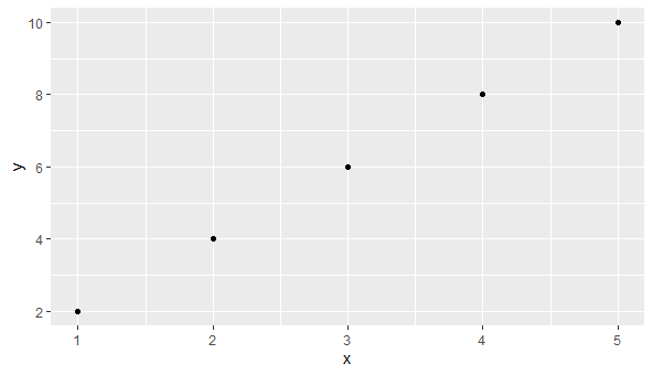
ggplot

21. What are the main features of the Dplyr package?

A powerful package for data manipulation in R is called dplyr. It offers a number of features that make efficient and simple data manipulation jobs possible. The dplyr package’s primary attributes and capabilities are listed below:

• Data Manipulation Verbs
• Chaining Operations
• Support for Various Data Sources
• Easy Joining of Data Frames
• Efficient Backend Optimization

22. How to Concatenate Strings in R?

In R, there are multiple ways to concatenate strings. Here are three commonly used methods:

Using the paste() function: The paste() function joins strings together, by default separating each string with a space. To concatenate several strings, use paste() with multiple arguments.

R

# Concatenate strings using paste()
string1 <- "Hello"
string2 <- "Geeks!"
result <- paste(string1, string2)
print(result)

Output:

[1] "Hello Geeks!"

Using the sprintf() function: We can format and concatenate strings using placeholders with the sprintf() method. When we want to control the format of the concatenated string.

R

# Concatenate strings using sprintf()
string1 <- "Hello"
string2 <- "Geeks!"
result <- sprintf("%s %s", string1, string2)
print(result)

Output:

[1] "Hello Geeks!"

In the example above, %s is a placeholder that gets replaced by the respective strings when using sprintf().

23. Explain how to handle missing data

Handling missing data is an important step in data preprocessing and analysis. Here are some common approaches to handling missing data in R.

• Identify Missing Data: The first step is to locate any missing values in our dataset. Missing values in R are often shown as NA. You can identify missing values in your data by using functions like complete. cases() and is.na().
• Remove Missing Data: We can just delete the rows or columns containing missing data if the dataset only has a small number of missing values and doing so won’t have a big impact on the analysis. Rows that have any missing values can be removed using the na.omit() function.

# Remove rows with missing values
clean_data <- na.omit(our_data)

R Interview Questions for Experienced

24. How to plot the heatmap of the correlation matrix in R?

• First, Use the cor() function to calculate the correlation matrix of your data.
• Ensure that our data is in a suitable format, such as a data frame or matrix, with numerical variables. we may need to preprocess or select a subset of variables for correlation analysis.
• Use the heatmap() function to create the heatmap.

25. How to make multiple plots in R?

To make multiple plots in R, you can use various techniques depending on your requirements. Here are two common approaches:

1. Using the layout() Function: Multiple plots can be arranged with additional flexibility using the layout() function. we can create a personalized layout with various sizes and configurations for each plot.
2. Using External Packages: The external R packages ggplot2, gridExtra, and cowplot all offer more sophisticated capabilities for making numerous charts. These packages provide customizable themes, versatile arrangements, and extra capabilities for building many plots that look good.

26. Create a 3D plot in R.

Typically used to illustrate the relationship between three variables, a 3D plot in R is a three-dimensional graphic representation of data. It enables us to investigate and comprehend intricate data linkages and patterns that are difficult to visualize in conventional 2D graphs.

The rgl package in R can be used to generate 3D plots. An adaptable and engaging environment for creating 3D visualizations is offered by this suite. The main steps in developing a 3D plot are as follows:

R

library(rgl)

# Create example data
x <- c(1, 2, 3, 4, 5)
y <- c(2, 4, 6, 8, 10)
z <- c(3, 6, 9, 12, 15)

# Create a 3D scatter plot
plot3d(x, y, z, type = "s", size = 2, col = "blue",
xlab = "X", ylab = "Y", zlab = "Z",
main = "3D Scatter Plot")

Output:

3D Plot

The plot3d() function is used to create the 3D scatter plot. It takes the x, y, and z coordinates as inputs and allows you to specify various parameters to customize the plot.

27. How to merge data?

In R, we can merge data using different functions, depending on the type of merge operation we want to perform and the structure of our data. Here are three common methods for merging data in R:

1. Merge using merge(): We can join data frames using the merge() function based on shared columns or variables. By default, it does an inner join, which means that the merged result will only contain the matching rows from the two data frames.
   
2. Merge using cbind() or rbind(): The cbind() or rbind() functions can be used to merge data frames by merely inserting columns or rows, respectively. These functions concatenate columns (cbind()) or rows (rbind()) of data frames without doing any key-based matching.
   
3. Merge using dplyr package: Data frame merging is among the data manipulation tools offered by the dplyr package. Similar to merge(), the dplyr functions inner_join(), left_join(), right_join(), and full_join() let we conduct various join kinds.

28. Explain the five statistical measures which are used in Boxplot.

In R, the boxplot() function is used to create boxplots. Boxplots are a graphical representation of the distribution of a dataset, showing the median, quartiles, and potential outliers. Or  A box graph is a chart that is used to display information in the form of distribution by drawing boxplots for each of them. This distribution of data is based on five sets (minimum, first quartile, median, third quartile, and maximum).

R

# Create a numeric vector
data <- c(1, 2, 3, 4, 5, 6, 7, 8, 9, 10)

# Create a boxplot
boxplot(data)

Output:

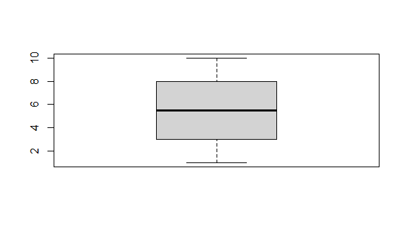
Box Plot

29. What is the difference between lapply and sapply?

Both lapply() and sapply() are functions in R that are used for applying a function to elements of a list or vector. However, there are some differences between the two:

lapply()	sapply()
Lapply() always produces a list with each entry representing the outcome of applying the function to each input element.	Simplifying the result into a vector, matrix, or array is one of the goals of the sapply() function. It will return a vector if the output is a scalar for each element. The output will produce a list if the lengths vary.
It is more adaptable and enables output structures with greater complexity. When we wish to keep the output’s list structure, we can utilize it.	Simplifying the output automatically with sapply() makes it more practical in simpler scenarios. If possible, it automatically converts the output to a vector, matrix, or array.
When we want to apply a function to each member of a list or vector and return the results as a list, the method lapply() is helpful.	When we want the result into a more practical format (vector, matrix, or array) if at all possible with the help of the sapply() function, which you can use to apply a function to each element of a list or vector.

30. How to add a title in plots of ggplot package?

To add a title to a plot created with the ggplot2 package in R, we can use the labs() function to modify the plot’s labels. Specifically, we can use the title argument to set the title of the plot.

# Customized title

   our_plot <- our_plot + labs(

  title = “our Plot Title”,
  size = 16,       # Font size
 color = “blue”,  # Font color
 fontface = “bold”  # Font style

)

# Display the plot
print(our_plot)

31. Explain rbind() and cbind() functions in R.

In R, rbind() and cbind() are functions used for combining or merging data objects vertically (rbind()) or horizontally (cbind()).

• rbind() function: Row adding is used to merge items using the function rbind(), which stands for “row bind”.
  Multiple objects can be passed to rbind(), which will stack them vertically according to their
  columns. The objects must have compatible column names or the same amount of columns.
• cbind() function: The “column bind” function, known as cbind(), is used to merge objects by appending columns.
  The function cbind() combines multiple objects horizontally by matching their rows. It accepts
  multiple inputs. The objects must have comparable row names or the same number of rows.

The fact that rbind() and cbind() are not restricted to data frames or vectors. Additionally, they can be used with many kinds of objects, such as arrays, lists, and matrices. However, for the functions to be effective, the objects being joined must have compatible rows or columns.

32. Explain Regularization in R.

Regularization is a form of regression technique that shrinks or regularizes or constrains the coefficient estimates towards 0 (or zero). In this technique, a penalty is added to the various parameters of the model in order to reduce the freedom of the given model. The concept of Regularization can be broadly classified into:

• Ridge Regression
• Lasso Regression
• Elastic Net Regression

In the R language, to perform Regularization we need a handful of packages to be installed before we start working on them. The required packages are 

• glmnet package for ridge regression and lasso regression
• dplyr package for data cleaning
• psych package in order to perform or compute the trace function of a matrix
• caret package

33. Explain the Lattice package.

A well-liked R tool for data visualization called lattice offers a robust and adaptable foundation for making trellis plots. It allows us to analyze large datasets and visualize multivariate relationships because it is based on conditioning and paneling concepts.

# Load the lattice package
library(lattice)
# Create a scatter plot
xyplot(y ~ x | group, data = our_data, type = "p", auto.key = TRUE)

The lattice package offers a wide range of functions and options for designing trellis plots that can be completely customized. We can use lattice to the fullest extent possible for visualizing complex datasets and investigating multivariate relationships by investigating the documentation and examples.

34. What is data normalization in R?

The process of converting numerical data into a common scale in order to remove magnitude disparities and bring the data to a standard range is known as data normalization, also known as data standardization or feature scaling. In many jobs involving data analysis and machine learning, it is an essential preprocessing step.

The data are scaled to a particular range or distribution during normalization. There are numerous normalization methods, including unit vector normalization, decimal scaling, and logarithmic normalization. The right approach will differ depending on the data and the intended normalization objective.

35. Explain some packages which are used in data mining.

The extraction of useful knowledge and insights from huge databases is the focus of the multidisciplinary area of data mining. Several R packages are frequently utilized for data mining activities. Here are some well-liked packages for data mining:

1. caret (Classification and Regression Training)
2. e1071
3. randomForest
4. cluster
5. tm (Text Mining)
6. ROCR

These are just a few examples of the many packages available for data mining in R. Depending on the specific task and requirements, you may find additional packages that cater to your needs. It’s always recommended to explore the documentation and examples of each package to understand their functionalities and how they can be effectively utilized for data mining tasks.

36. How to handle outliers?

For statistical analyses and machine learning models to be accurate and reliable, handling outliers is a crucial step in the preparation of the data. These typical methods for handling outliers in your data are listed below:

Recognize Outliers

Determine any potential outliers in your dataset first. To visually check the data for any extreme values, one typical strategy is to utilize graphical techniques like box plots, scatter plots, or histograms. Statistical tools like the z-score and the interquartile range (IQR) can also be used to find outliers.

Remove Outliers

If the outliers are the result of measurement errors or errors in data input and are not likely to represent true values, you might want to remove them from the dataset. The removal of outliers must be done carefully, though, as they can lead to other problems.

37. Explain time series analysis and how to perform it in R.

Data that is gathered and recorded across a series of time intervals can be analyzed and modeled using a statistical technique called time series analysis. In order to anticipate or derive insights for future time points, it focuses on analyzing the patterns, trends, and dependencies within the data. Numerous disciplines, including finance, economics, environmental sciences, and demand forecasting, heavily rely on time series analysis.

For time series analysis in R, there are a number of packages and functions. Here is a summary of the main steps in conducting a time series analysis in R:

• Loading Time Series Data
• Data Exploration and Visualization
• Time Series Decomposition
• Stationarity Testing
• Time Series Modeling
• Model Evaluation and Selection
• Forecasting
• Model Diagnostics and Residual Analysis

Forecast, xts, zoo, and tsibble are just a few of the time series analysis-specific packages available in R. To handle several facets of time series analysis, such as data manipulation, modeling, visualization, and forecasting, these packages provide a wide range of features and tools.

38. How to create a decision tree in R?

The CART (Classification and Regression Trees) technique is implemented by the rpart package in R, and it can be used to build decision trees. The rpart package offers tools for creating and visualizing decision tree models. An instruction manual for building a decision tree in R is provided below:

R

# Load the required packages
library(rpart)
library(rpart.plot)

# Load the mtcars dataset
data(mtcars)

# Build the decision tree model
tree_model <- rpart(vs ~ mpg + cyl + hp + wt,
data = mtcars)

# Plot the decision tree using rpart.plot
rpart.plot(tree_model, box.palette = "Blues",
shadow.col = "gray", nn = TRUE)

Output:

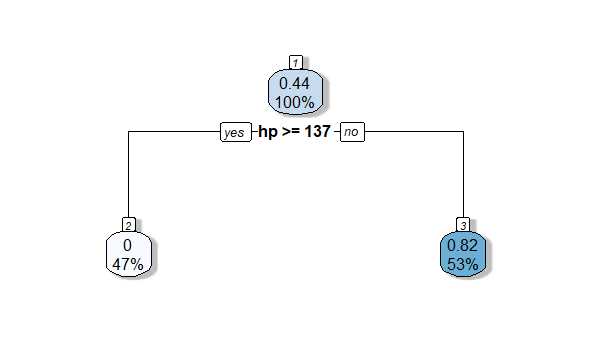
RPlot

39. What is a p-value in hypothesis testing, and how can you calculate it in R?

The p-value in hypothesis testing is a gauge of the weight of the evidence against the null hypothesis. It displays the likelihood of witnessing the test statistic (or a more extreme number) if the null hypothesis is accepted. In other words, it measures the probability that the observed data would be obtained if the null hypothesis were true.

To calculate the p-value in R, we use functions from statistical packages. Here’s an example using the t.test() function from the stats package to calculate the p-value for a two-sample t-test:

R

# Example data
group1 <- c(1, 2, 3, 4, 5)
group2 <- c(2, 4, 6, 8, 10)

# Perform two-sample t-test
result <- t.test(group1, group2)

# Extract the p-value
p_value <- result$p.value

# Print the p-value
print(p_value)

Output:

[1] 0.1075312

40. Explain the chi-squared test in R.

A statistical test called the chi-squared test is used to detect if category variables are significantly associated. It is frequently used in conjunction with contingency tables, which show the frequencies or counts of various categories for two or more variables.

In R, you can perform the chi-squared test using the chistest() function.

Output:

    Pearson's Chi-squared test with Yates' continuity correction
data:  a1
X-squared = 0.00058442, df = 1, p-value = 0.9807

41. Difference between correlation and PCA?

Both correlation and Principal Component Analysis (PCA), statistical methods used in data analysis, have distinct objectives and yield unique insights. Here is a quick description of each:

correlation	PCA
The strength and direction of the linear link between two variables are measured by correlation. It measures how closely connected the variables are to one another.	By breaking complicated datasets down into a more manageable group of uncorrelated variables known as principal components, PCA is a dimensionality reduction technique used to make complex datasets simpler.
Typically, correlation is expressed by a number between -1 and 1. As one variable rises, the other tends to rise as well. A positive number denotes a positive correlation, a negative value denotes a negative correlation, and a value near to zero denotes a weak or nonexistent link.	PCA identifies the linear combinations of the initial variables that best capture the range of the data. The greatest substantial amount of variation is explained by the first principal component, then by the second, and so on.
Understanding the correlation between two variables and evaluating the strength of their linear relationship are both possible through correlation. It aids in the discovery of patterns, interdependence, and possible cause-and-effect connections.	When working with high-dimensional datasets, PCA is especially helpful for locating underlying structures, lowering noise, and enhancing the data’s readability.

In conclusion, correlation measures the strength and direction of the linear association between two variables and focuses on the relationship between them. The PCA method, on the other hand, is a feature extraction and dimensionality reduction method that aids in locating the most crucial patterns and reducing the complexity of high-dimensional datasets.

42. Explain linear regression and how to perform it in R.

A statistical modeling method called linear regression is employed to determine the relationship between a dependent variable and one or more independent variables. The variables are assumed to be related linearly, with changes in the independent variables translating into proportional changes in the dependent variable.

To perform linear regression in R, we can follow these steps:

• Data Preparation.
• Load the Data.
• Inspect the Data.
• Build the Linear Regression Model.
• Analyze the Model.
• Make Predictions.

43. What is logistic regression?

A statistical modeling method called logistic regression is used to estimate the likelihood of a binary outcome based on one or more independent factors. When the dependent variable is categorical (binary or dichotomous), logistic regression is employed instead of linear regression, which forecasts continuous values.

Analysis and evaluation techniques, such as assessing model fit and evaluating the model’s predictive performance, can be employed to gain more insights and validate the logistic regression model.

44. How to perform cross-validation?

A predictive model’s performance is evaluated using the cross-validation technique, which divides the available data into training and validation sets. Estimating how well the model will apply to fresh, untested data is helpful. Here is a general description of cross-validation:

• Data Preparation.
• Choose the Number of Folds.
• Partition the Data.
• Model Training and Evaluation.
• Model Selection and Improvement.

It’s important to note that R offers a number of packages and methods to make cross-validation easier, like caret, rsample, and tidymodels. Within the cross-validation framework, these packages provide simple ways to divide the data into different groups, train models, and calculate performance indicators.

45. Explain feature selection and some packages in R which can help us achieve this. 

The process of picking the most pertinent and instructive subset of features (independent variables) from a larger set of features in a dataset is known as feature selection, also known as variable selection or attribute selection. By deleting pointless or superfluous characteristics from the model, feature selection aims to optimize model performance, eliminate overfitting, improve interpretability, and reduce computing complexity.
There are several methods for feature selection:

1. Filter Methods.
2. Wrapper Methods.
3. Embedded Methods.

In R, there are several packages that provide useful functions for feature selection. Here are a few popular ones:

• caret
• boruta
• glmnet
• randomForest

These tools provide a variety of feature selection methods and procedures to assist us in finding pertinent characteristics in our data. our dataset’s unique properties and the objectives of our research will influence.

46. What is the ROC curve and how to plot it in R?

A binary classification model’s effectiveness is graphically represented by the ROC (Receiver Operating Characteristic) curve. It demonstrates how, at different categorization thresholds, the true positive rate (sensitivity) and the false positive rate(specificity1) trade-off.

To plot a ROC curve in R, you can follow these steps:

1. Obtain Predicted Probabilities.
2. Load Necessary Packages.
3. Compute ROC Curve.
4. Plot ROC Curve.

R

# Install and load the pROC package
install.packages("pROC")
library(pROC)

# Simulated example data
a1 <- c(1, 0, 1, 1, 0, 1)
a2 <- c(0.3, 0.4, 0.5, 0.6, 0.7, 0.8)

# Compute ROC curve
plot_r <- roc(a1, a2)

# Plot ROC curve
plot(plot_r)

Output:

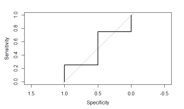
ROC Curve

47. How to calculate the accuracy of R models?

To calculate the accuracy of R models, we typically compare the predicted values from the model to the true values in our dataset. The accuracy metric is defined as the proportion of correct predictions made by the model.

We use the confusionMatrix function from the caret package to mapping the accuracy of models. Here is a small example.

R

# Simulated example data
a1 <- c(1, 0, 1, 0, 1)
a2 <- c(1, 0, 1, 1, 0)

# Calculate the accuracy
confusionMatrix(factor(a1),factor(a2))

Output:

Confusion Matrix and Statistics
          Reference
Prediction 0 1
         0 1 1
         1 1 2
                                          
               Accuracy : 0.6             
                 95% CI : (0.1466, 0.9473)
    No Information Rate : 0.6             
    P-Value [Acc > NIR] : 0.6826          
                                          
                  Kappa : 0.1667          
                                          
 Mcnemar's Test P-Value : 1.0000          
                                          
            Sensitivity : 0.5000          
            Specificity : 0.6667          
         Pos Pred Value : 0.5000          
         Neg Pred Value : 0.6667          
             Prevalence : 0.4000          
         Detection Rate : 0.2000          
   Detection Prevalence : 0.4000          
      Balanced Accuracy : 0.5833          
                                          
       'Positive' Class : 0                          

48. How do you optimize parameters in machine learning models in R?

In R, methods like grid search, random search, or more complex optimization algorithms are frequently used to optimize parameters in machine learning models. from this, we are able to methodically investigate various parameter value combinations in search of the ideal collection of parameters that will maximize the performance of our model.

Here’s a general step to optimizing parameters in R:

1. Define Parameter Grid.
2. Choose Evaluation Metric.
3. Perform Cross-Validation.
4. Select Optimal Parameters.
5. Evaluation of the Test Set.

By following these steps we optimize parameters in machine learning models in R.

49. What is ntree function?

ntree function belongs to the RandomForest package in R. The ntree parameter in the context of random forests normally denotes the number of decision trees to be grown in the ensemble of the random forest. An ensemble learning technique called random forests combines various decision trees to produce predictions. The ntree parameter defines the number of trees to be included in the ensemble. Each decision tree is trained on a random subset of the training data.

For instance, the randomForest() function in the R randomForest package uses the ntree parameter to determine the number of trees to be created.

50. What is glm in R?

glm() function in R Language is used to fit linear models to the dataset. Here, glm stands for a generalized linear model. It is a flexible tool for doing a variety of statistical analyses and response variables using a variety of distributions and link functions.

glm(formula, data, family, ...)

• formula: This argument specifies the model formula, where you define the relationship between the response variable and the predictor variable
• data: The data frame containing the variables utilized in the model is specified by this argument.
• family: The generalized linear model’s distributional family and link function are specified by this argument. The terms “Gaussian” (for linear regression), “binomial” (for logistic regression), “poisson” (for Poisson regression), and “gamma” (for gamma regression) are a few of the often used families.

Conclusion

In conclusion, the top 50 R interview questions and answers, covered a wide range of topics, from data wrangling and statistical analysis to machine learning and visualization. By familiarizing yourself with these questions, you can increase your chances of success in your next R interview.