Python Bokeh is a Data Visualization library that provides interactive charts and plots. Bokeh renders its plots using HTML and JavaScript that uses modern web browsers for presenting elegant, concise construction of novel graphics with high-level interactivity.
Features of Bokeh:
- Flexibility: Bokeh can be used for common plotting requirements and for custom and complex use-cases.
- Productivity: Its interaction with other popular Pydata tools (such as Pandas and Jupyter notebook) is very easy.
- Interactivity: It creates interactive plots that change with the user interaction.
- Powerful: Generation of visualizations for specialized use-cases can be done by adding JavaScript.
- Shareable: Visual data are shareable. They can also be rendered in Jupyter notebooks.
- Open source: Bokeh is an open-source project.

This tutorial aims at providing insight to Bokeh using well-explained concepts and examples with the help of a huge dataset. So let’s dive deep into the Bokeh and learn all it from basic to advance.
Table Of Content
Installation
Bokeh is supported by CPython 3.6 and older with both standard distribution and anaconda distribution. Bokeh package has the following dependencies.
1. Required Dependencies
- PyYAML>=3.10
- python-dateutil>=2.1
- Jinja2>=2.7
- numpy>=1.11.3
- pillow>=4.0
- packaging>=16.8
- tornado>=5
- typing_extensions >=3.7.4
2. Optional Dependencies
- Jupyter
- NodeJS
- NetworkX
- Pandas
- psutil
- Selenium, GeckoDriver, Firefox
- Sphinx
Bokeh can be installed using both conda package manager and pip. To install it using conda type the below command in the terminal.
conda install bokeh
This will install all the dependencies. If all the dependencies are installed then you can install the bokeh from PyPI using pip. Type the below command in the terminal.
pip install bokeh
Refer to the below article to get detailed information about the installation of Bokeh.
Bokeh Interfaces – Basic Concepts of Bokeh
Bokeh is simple to use as it provides a simple interface to the data scientists who do not want to be distracted by its implementation and also provides a detailed interface to developers and software engineers who may want more control over the Bokeh to create more sophisticated features. To do this Bokeh follows the layered approach.
Bokeh.models
This class is the Python Library for Bokeh that contains model classes that handle the JSON data created by Bokeh’s JavaScript library (BokehJS). Most of the models are very basic consisting of very few attributes or no methods.
bokeh.plotting
This is the mid-level interface that provides Matplotlib or MATLAB like features for plotting. It deals with the data that is to be plotted and creating the valid axes, grids, and tools. The main class of this interface is the Figure class.
Getting Started
After the installation and learning about the basic concepts of Bokeh let’s create a simple plot.
Example:
Python3
from bokeh.plotting import figure, output_file, show
graph = figure(title = "Bokeh Line Graph")
x = [1, 2, 3, 4, 5]
y = [5, 4, 3, 2, 1]
graph.line(x, y)
show(graph)
|
Output:
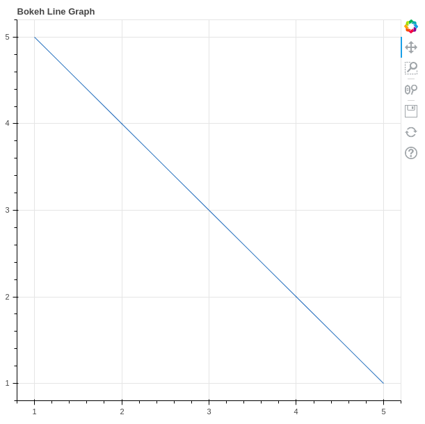
In the above example, we have created a simple Plot with the Title as Bokeh Line Graph. If you are using Jupyter then the output will be created in a new tab in the browser.
Annotations and Legends
Annotations are the supplemental information such as titles, legends, arrows, etc that can be added to the graphs. In the above example, we have already seen how to add the titles to the graph. In this section, we will see about the legends.
Adding legends to your figures can help to properly describe and define them. Hence, giving more clarity. Legends in Bokeh are simple to implement. They can be basic, automatically grouped, manually mentioned, explicitly indexed, and also interactive.
Example:
Python3
from bokeh.plotting import figure, output_file, show
graph = figure(title="Bokeh Line Graph")
x = [1, 2, 3, 4, 5]
y = [5, 4, 3, 2, 1]
graph.line(x, x, legend_label="Line 1")
graph.line(y, x, legend_label="Line 2",
line_color="green")
show(graph)
|
Output:
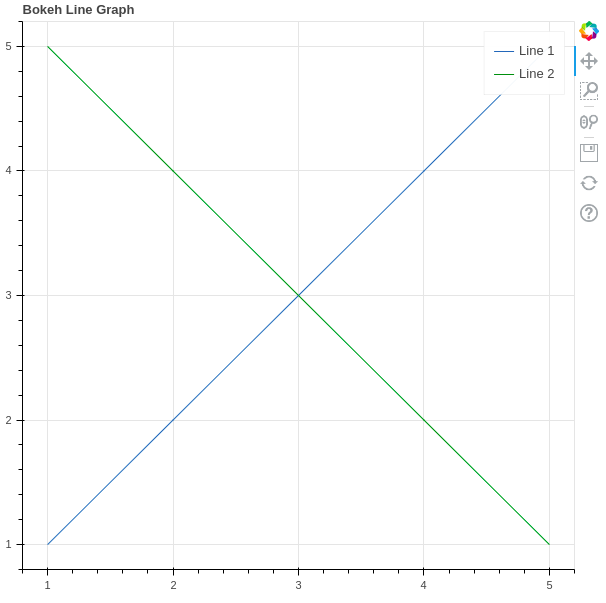
In the above example, we have plotted two different lines with a legend that simply states that which is line 1 and which is line 2. The color in the legends is also differentiated by the color.
Refer to the below articles to get detailed information about the annotations and legends
Customizing Legends
Legends in Bokeh can be customized using the following properties.
| Property |
Description |
| legend.label_text_font |
change default label font to specified font name |
| legend.label_text_font_size |
font size in points |
| legend.location |
set the label at specified location. |
| legend.title |
set title for legend label |
| legend.orientation |
set to horizontal (default) or vertical |
| legend.clicking_policy |
specify what should happen when legend is clicked |
Example:
Python3
from bokeh.plotting import figure, output_file, show
graph = figure(title="Bokeh Line Graph")
x = [1, 2, 3, 4, 5]
y = [5, 4, 3, 2, 1]
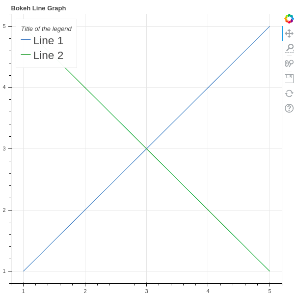
graph.line(x, x, legend_label="Line 1")
graph.line(y, x, legend_label="Line 2",
line_color="green")
graph.legend.title = "Title of the legend"
graph.legend.location ="top_left"
graph.legend.label_text_font_size = "17pt"
show(graph)
|
Output:
Plotting Different Types of Plots
Glyphs in Bokeh terminology means the basic building blocks of the Bokeh plots such as lines, rectangles, squares, etc. Bokeh plots are created using the bokeh.plotting interface which uses a default set of tools and styles.
Line Plot
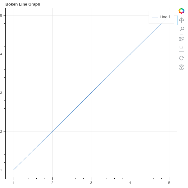
Line charts are used to represent the relation between two data X and Y on a different axis. A line plot can be created using the line() method of the plotting module.
Syntax:
line(parameters)
Example:
Python3
from bokeh.plotting import figure, output_file, show
graph = figure(title = "Bokeh Line Graph")
x = [1, 2, 3, 4, 5]
y = [5, 4, 3, 2, 1]
graph.line(x, y)
show(graph)
|
Output:
Refer to the below articles to get detailed information about the line plots.
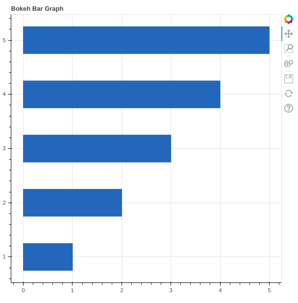
Bar Plot
Bar plot or Bar chart is a graph that represents the category of data with rectangular bars with lengths and heights that is proportional to the values which they represent. It can be of two types horizontal bars and vertical bars. Each can be created using the hbar() and vbar() functions of the plotting interface respectively.
Syntax:
hbar(parameters)
vbar(parameters)
Example 1: Creating horizontal bars.
Python3
from bokeh.plotting import figure, output_file, show
graph = figure(title = "Bokeh Bar Graph")
x = [1, 2, 3, 4, 5]
y = [1, 2, 3, 4, 5]
height = 0.5
graph.hbar(x, right = y, height = height)
show(graph)
|
Output:
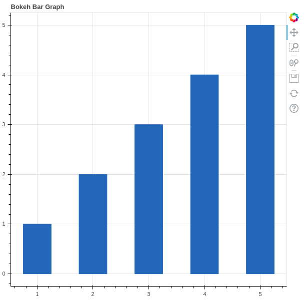
Example 2: Creating the vertical bars
Python3
from bokeh.plotting import figure, output_file, show
graph = figure(title = "Bokeh Bar Graph")
x = [1, 2, 3, 4, 5]
y = [1, 2, 3, 4, 5]
width = 0.5
graph.vbar(x, top = y, width = width)
show(graph)
|
Output:
Refer to the below articles to get detailed information about the bar charts.
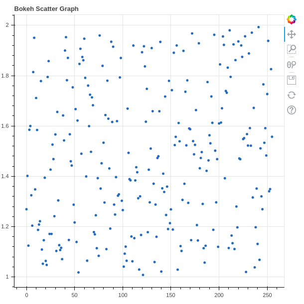
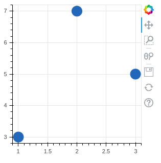
Scatter Plot
A scatter plot is a set of dotted points to represent individual pieces of data in the horizontal and vertical axis. A graph in which the values of two variables are plotted along X-axis and Y-axis, the pattern of the resulting points reveals a correlation between them. It can be plotted using the scatter() method of the plotting module.
Syntax:
scatter(parameters)
Example:
Python3
from bokeh.plotting import figure, output_file, show
from bokeh.palettes import magma
import random
graph = figure(title = "Bokeh Scatter Graph")
x = [n for n in range(256)]
y = [random.random() + 1 for n in range(256)]
graph.scatter(x, y)
show(graph)
|
Output:
Refer to the below articles to get detailed information about the scatter plots.
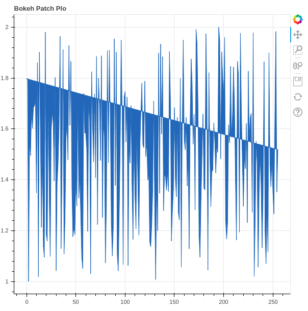
Patch Plot
Patch Plot shades a region of area to show a group having same properties. It can be created using the patch() method of the plotting module.
Syntax:
patch(parameters)
Example:
Python3
from bokeh.plotting import figure, output_file, show
from bokeh.palettes import magma
import random
graph = figure(title = "Bokeh Patch Plo")
x = [n for n in range(256)]
y = [random.random() + 1 for n in range(256)]
graph.patch(x, y)
show(graph)
|
Output:
Refer to the below articles to get detailed information about the Patch Plot.
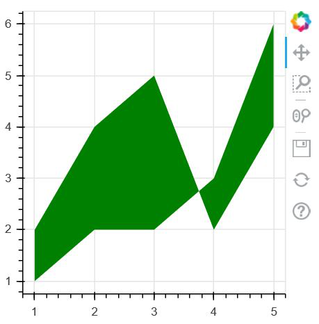
Area Plot
Area plots are defined as the filled regions between two series that share a common areas. Bokeh Figure class has two methods which are – varea(), harea()
Syntax:
varea(x, y1, y2, **kwargs)
harea(x1, x2, y, **kwargs)
Example 1: Creating vertical area plot
Python
import numpy as np
from bokeh.plotting import figure, output_file, show
x = [1, 2, 3, 4, 5]
y1 = [2, 4, 5, 2, 4]
y2 = [1, 2, 2, 3, 6]
p = figure(plot_width=300, plot_height=300)
p.varea(x=x, y1=y1, y2=y2,fill_color="green")
show(p)
|
Output:
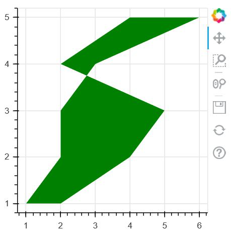
Example 2: Creating horizontal area plot
Python3
import numpy as np
from bokeh.plotting import figure, output_file, show
y = [1, 2, 3, 4, 5]
x1 = [2, 4, 5, 2, 4]
x2 = [1, 2, 2, 3, 6]
p = figure(plot_width=300, plot_height=300)
p.harea(x1=x1, x2=x2, y=y,fill_color="green")
show(p)
|
Output:
Refer to the below articles to get detailed information about the area charts
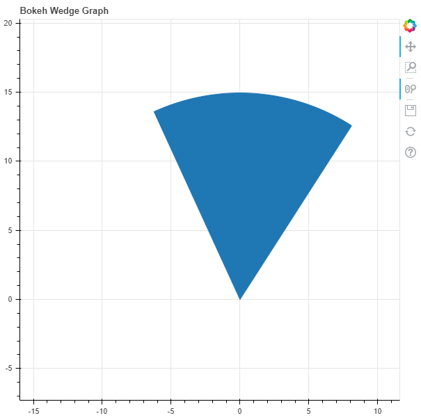
Pie Chart
Bokeh Does not provide a direct method to plot the Pie Chart. It can be created using the wedge() method. In the wedge() function, the primary parameters are the x and y coordinates of the wedge, the radius, the start_angle and the end_angle of the wedge. In order to plot the wedges in such a way that they look like a pie chart, the x, y, and radius parameters of all the wedges will be the same. We will only adjust the start_angle and the end_angle.
Syntax:
wedge(parameters)
Example:
Python3
from bokeh.plotting import figure, output_file, show
graph = figure(title = "Bokeh Wedge Graph")
x = 0
y = 0
radius = 15
start_angle = 1
end_angle = 2
graph.wedge(x, y, radius = radius,
start_angle = start_angle,
end_angle = end_angle)
show(graph)
|
Output:
Refer to the below articles to get detailed information about the pie charts.
Creating Different Shapes
The Figure class in Bokeh allows us create vectorised glyphs of different shapes such as circle, rectangle, oval, polygon, etc. Let’s discuss them in detail.
Circle
Bokeh Figure class following methods to draw circle glyphs which are given below:
- circle() method is a used to add a circle glyph to the figure and needs x and y coordinates of its center.
- circle_cross() method is a used to add a circle glyph with a ‘+’ cross through the center to the figure and needs x and y coordinates of its center.
- circle_x() method is a used to add a circle glyph with a ‘X’ cross through the center. to the figure and needs x and y coordinates of its center.
Example:
Python3
import numpy as np
from bokeh.plotting import figure, output_file, show
plot = figure(plot_width = 300, plot_height = 300)
plot.circle(x = [1, 2, 3], y = [3, 7, 5], size = 20)
show(plot)
|
Output:
Refer to the below articles to get detailed information about the circle glyphs
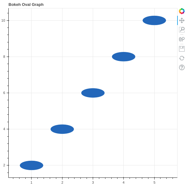
Oval
oval() method can be used to plot ovals on the graph.
Syntax:
oval(parameters)
Example:
Python3
from bokeh.plotting import figure, output_file, show
graph = figure(title = "Bokeh Oval Graph")
x = [1, 2, 3, 4, 5]
y = [i * 2 for i in x]
graph.oval(x, y,
height = 0.5,
width = 1)
show(graph)
|
Output:
Refer o the below articles to get detailed information about the oval glyphs.
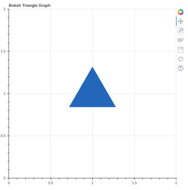
Triangle
Triangle can be created using the triangle() method.
Syntax:
triangle(parameters)
Example:
Python3
from bokeh.plotting import figure, output_file, show
graph = figure(title = "Bokeh Triangle Graph")
x = 1
y = 1
graph.triangle(x, y, size = 150)
show(graph)
|
Output:
Refer to the below article to get detailed information about the triangles.
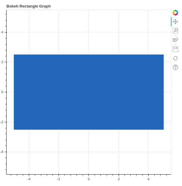
Rectangle
Just like circles and ovals rectangle can also be plotted in Bokeh. It can be plotted using the rect() method.
Syntax:
rect(parameters)
Example:
Python3
from bokeh.plotting import figure, output_file, show
graph = figure(title = "Bokeh Rectangle Graph", match_aspect = True)
x = 0
y = 0
width = 10
height = 5
graph.rect(x, y, width, height)
show(graph)
|
Output:
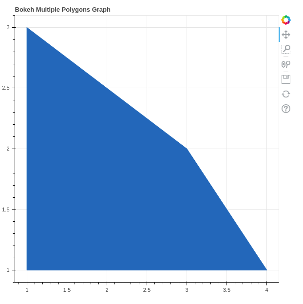
Polygon
Bokeh can also be used to plot multiple polygons on a graph. Plotting multiple polygons on a graph can be done using the multi_polygons() method of the plotting module.
Syntax:
multi_polygons(parameters)
Example:
Python3
from bokeh.plotting import figure, output_file, show
graph = figure(title = "Bokeh Multiple Polygons Graph")
xs = [[[[1, 1, 3, 4]]]]
ys = [[[[1, 3, 2 ,1]]]]
graph.multi_polygons(xs, ys)
show(graph)
|
Output:
Refer to the below articles to get detailed information about the polygon glyphs.
Plotting Multiple Plots
There are several layouts provided by the Bokeh in order to create Multiple Plots. These layouts are:
- Vertical Layout
- Horizontal Layout
- Grid Layout
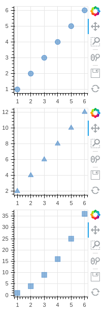
Vertical Layouts
Vertical Layout set all the plots in the vertical fashion and can be created using the column() method.
Python3
from bokeh.io import output_file, show
from bokeh.layouts import column
from bokeh.plotting import figure
x = [1, 2, 3, 4, 5, 6]
y0 = x
y1 = [i * 2 for i in x]
y2 = [i ** 2 for i in x]
s1 = figure(width=200, plot_height=200)
s1.circle(x, y0, size=10, alpha=0.5)
s2 = figure(width=200, height=200)
s2.triangle(x, y1, size=10, alpha=0.5)
s3 = figure(width=200, height=200)
s3.square(x, y2, size=10, alpha=0.5)
p = column(s1, s2, s3)
show(p)
|
Output:
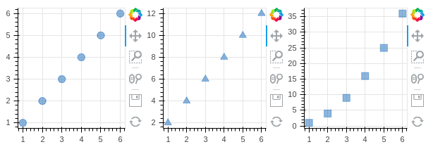
Horizontal Layout
Horizontal Layout set all the plots in the horizontal fashion. It can be created using the row() method.
Example:
Python3
from bokeh.io import output_file, show
from bokeh.layouts import row
from bokeh.plotting import figure
x = [1, 2, 3, 4, 5, 6]
y0 = x
y1 = [i * 2 for i in x]
y2 = [i ** 2 for i in x]
s1 = figure(width=200, plot_height=200)
s1.circle(x, y0, size=10, alpha=0.5)
s2 = figure(width=200, height=200)
s2.triangle(x, y1, size=10, alpha=0.5)
s3 = figure(width=200, height=200)
s3.square(x, y2, size=10, alpha=0.5)
p = row(s1, s2, s3)
show(p)
|
Output:
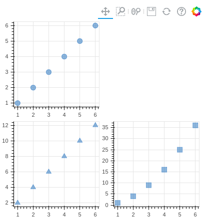
Grid Layout
gridplot() method can be used to arrange all the plots in the grid fashion. we can also pass None to leave a space empty for a plot.
Example:
Python3
from bokeh.io import output_file, show
from bokeh.layouts import gridplot
from bokeh.plotting import figure
x = [1, 2, 3, 4, 5, 6]
y0 = x
y1 = [i * 2 for i in x]
y2 = [i ** 2 for i in x]
s1 = figure()
s1.circle(x, y0, size=10, alpha=0.5)
s2 = figure()
s2.triangle(x, y1, size=10, alpha=0.5)
s3 = figure()
s3.square(x, y2, size=10, alpha=0.5)
p = gridplot([[s1, None], [s2, s3]], plot_width=200, plot_height=200)
show(p)
|
Output:
Interactive Data Visualization
One of the key feature of Bokeh which differentiate it from other visualizing libraries is adding interaction to the Plot. Let’s see various interactions that can be added to the plot.
Configuring Plot Tools
In all the above graphs you must have noticed a toolbar that appears mostly at the right of the plot. Bokeh provides us the methods to handle these tools. Tools can be classified into four categories.
- Gestures: These tools handle the gestures such as pan movement. There are three types of gestures:
- Pan/Drag Tools
- Click/Tap Tools
- Scroll/Pinch Tools
- Actions: These tools handle when a button is pressed.
- Inspectors: These tools report information or annotate the graph such as HoverTool.
- Edit Tools: These are multi gestures tools that can add, delete glyphs from the graph.
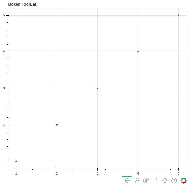
Adjusting the Position of the ToolBar
We can specify the position of the toolbar according to our own needs. It can be done by passing the toolbar_location parameter to the figure() method. The possible value to this parameter is –
- “above”
- “below”
- “left”
- “right”
Example:
Python3
from bokeh.plotting import figure, output_file, show
graph = figure(title = "Bokeh ToolBar", toolbar_location="below")
x = [1, 2, 3, 4, 5]
y = [1, 2, 3, 4, 5]
width = 0.5
graph.scatter(x, y)
show(graph)
|
Output:
In the section annotations and legends we have seen the list of all the parameters of the legends, however, we have not discussed the click_policy parameter yet. This property makes the legend interactive. There are two types of interactivity –
- Hiding: Hides the Glyphs.
- Muting: Hiding the glyph makes it vanish completely, on the other hand, muting the glyph just de-emphasizes the glyph based on the parameters.
Example 1: Hiding the legend
Python3
from bokeh.plotting import figure, output_file, show
output_file("gfg.html")
graph = figure(title = "Bokeh Hiding Glyphs")
graph.vbar(x = 1, top = 5,
width = 1, color = "violet",
legend_label = "Violet Bar")
graph.vbar(x = 2, top = 5,
width = 1, color = "green",
legend_label = "Green Bar")
graph.vbar(x = 3, top = 5,
width = 1, color = "yellow",
legend_label = "Yellow Bar")
graph.vbar(x = 4, top = 5,
width = 1, color = "red",
legend_label = "Red Bar")
graph.legend.click_policy = "hide"
show(graph)
|
Output:
Example 2: Muting the legend
Python3
from bokeh.plotting import figure, output_file, show
output_file("gfg.html")
graph = figure(title = "Bokeh Hiding Glyphs")
graph.vbar(x = 1, top = 5,
width = 1, color = "violet",
legend_label = "Violet Bar",
muted_alpha=0.2)
graph.vbar(x = 2, top = 5,
width = 1, color = "green",
legend_label = "Green Bar",
muted_alpha=0.2)
graph.vbar(x = 3, top = 5,
width = 1, color = "yellow",
legend_label = "Yellow Bar",
muted_alpha=0.2)
graph.vbar(x = 4, top = 5,
width = 1, color = "red",
legend_label = "Red Bar",
muted_alpha=0.2)
graph.legend.click_policy = "mute"
show(graph)
|
Output:
Adding Widgets to the Plot
Bokeh provides GUI features similar to HTML forms like buttons, slider, checkbox, etc. These provide an interactive interface to the plot that allows to change the parameters of the plot, modifying plot data, etc. Let’s see how to use and add some commonly used widgets.
- Buttons: This widget adds a simple button widget to the plot. We have to pass a custom JavaScript function to the CustomJS() method of the models class.
Syntax:
Button(label, icon, callback)
Example:
Python3
from bokeh.io import show
from bokeh.models import Button, CustomJS
button = Button(label="GFG")
button.js_on_click(CustomJS(
code="console.log('button: click!', this.toString())"))
show(button)
|
Output:

- CheckboxGroup: Adds a standard check box to the plot. Similarly to buttons we have to pass the custom JavaScript function to the CustomJS() method of the models class.
Example:
Python3
from bokeh.io import show
from bokeh.models import CheckboxGroup, CustomJS
L = ["First", "Second", "Third"]
checkbox_group = CheckboxGroup(labels=L, active=[0, 2])
checkbox_group.js_on_click(CustomJS(code=
))
show(checkbox_group)
|
Output:

- RadioGroup: Adds a simple radio button and accepts a custom JavaScript function.
Syntax:
RadioGroup(labels, active)
Example:
Python3
from bokeh.io import show
from bokeh.models import RadioGroup, CustomJS
L = ["First", "Second", "Third"]
radio_group = RadioGroup(labels=L, active=1)
radio_group.js_on_click(CustomJS(code=
))
show(radio_group)
|
Output:

- Sliders: Adds a slider to the plot. It also needs a custom JavaScript function.
Syntax:
Slider(start, end, step, value)
Example:
Python3
from bokeh.io import show
from bokeh.models import CustomJS, Slider
slider = Slider(start=1, end=20, value=1, step=2, title="Slider")
slider.js_on_change("value", CustomJS(code=
))
show(slider)
|
Output:
- DropDown: Adds a dropdown to the plot and like every other widget it also needs a custom JavaScript function as callback.
Example:
Python3
from bokeh.io import show
from bokeh.models import CustomJS, Dropdown
menu = [("First", "First"), ("Second", "Second"), ("Third", "Third")]
dropdown = Dropdown(label="Dropdown Menu", button_type="success", menu=menu)
dropdown.js_on_event("menu_item_click", CustomJS(
code="console.log('dropdown: ' + this.item, this.toString())"))
show(dropdown)
|
Output:
- Tab Widget: Tab Widget adds tabs and each tab show a different plot.
Example:
Python3
from bokeh.plotting import figure, output_file, show
from bokeh.models import Panel, Tabs
import numpy as np
import math
fig1 = figure(plot_width=300, plot_height=300)
x = [1, 2, 3, 4, 5]
y = [5, 4, 3, 2, 1]
fig1.line(x, y, line_color='green')
tab1 = Panel(child=fig1, title="Tab 1")
fig2 = figure(plot_width=300, plot_height=300)
fig2.line(y, x, line_color='red')
tab2 = Panel(child=fig2, title="Tab 2")
all_tabs = Tabs(tabs=[tab1, tab2])
show(all_tabs)
|
Output:
Creating Different Types of Glyphs
Visualizing Different Types of Data
More Topics on Bokeh
Share your thoughts in the comments
Please Login to comment...