Multiple linear regression using R for the Real estate data set

Multiple linear regression is widely used in machine learning and data science. In this article, We will discuss the Multiple linear regression by building a step-by-step project on a Real estate data set.

Multiple linear regression

Multiple Linear Regression is a statistical method used to model the relationship between a dependent variable (or target variable) and two or more independent variables (or predictor variables). It’s a valuable tool for understanding how multiple factors influence a particular outcome. In the context of real estate data, multiple linear regression can help us predict real estate prices based on various factors.

Here’s a step-by-step explanation of how to perform Multiple Linear Regression using R Programming Language for a Real Estate Sales dataset.

Multiple linear regression using R for the Real estate data set

Install the Required Libraries

Install xlsx R package

install.packages("xlsx")                                         

Load the Required Libraries

Before starting the analysis, you need to load the necessary R libraries. In this case, you might use libraries like readxl for reading data from Excel files and lm for fitting the regression model.

R

library("xlsx")

Load the Dataset

Dataset Link: REAL ESTATE SALES DATA

Import the Real Estate dataset into your R environment. You can use functions like read.xlsx or read.csv to read data from Excel or CSV files, respectively. Ensure that the dataset is structured with columns representing variables of interest, such as property price, size, number of bedrooms, number of bathrooms, and other relevant factors.

R

# Read xlsx file with read.xlsx
data<- read.xlsx("UNFILTERED DATA Vanderburgh  2013 PROPERTY SALES DATA.xlsx",
                   sheetIndex = 1)

head(data)

Output:

  OBJECTID              NAME                 StatePIN
1        1 12-180-34-217-037 82-05-12-034-217.037-020
2        2 10-080-18-116-003 82-05-23-018-116.003-025
3        3 11-350-25-040-006 82-06-20-025-040.006-029
4        4 11-440-26-059-013 82-06-20-026-059.013-029
5        5 09-610-16-049-002 82-06-33-016-049.002-027
6        6 11-020-20-050-014 82-06-30-020-050.014-029
                            legal_description       property_addr
1            SMITHLAND LOTS 37,38,39,40 BLK 1   3100 N FULTON AVE
2                  WESTHOLME LOTS 4 & 5 BLK 2 612 N ST JOSEPH AVE
3 HEIDELBACH & ELSAS ENLG LOTS 26 & 27 BLK 35    15 W FRANKLIN ST
4    GARVIN PARK LOTS 12 13 & PT LOT 14 BLK 7  216 E TENNESSEE ST
5                        WOODHAVEN LOTS 2 & 3     1403 MONROE AVE
6      EASTERN ENLARGEMENT PT L 13,14,15,BL 2     419 SE THIRD ST
  cert_land_value cert_improvement_value cert_total_value
1           30700                  21300            52000
2           43800                   3700            47500
3            9500                  37600            47100
4           10900                  54500            65400
5           15200                  80200            95400
6            6700                      0             6700
                          owner1 owner2             owner_street owner_city
1         TAYLOR, CHARLES ROBERT   <NA>         4810 TECUMSEH LN EVANSVILLE
2                 SCHMITT, STEVE   <NA>          3220 ORCHARD RD EVANSVILLE
3              SCHEESSELE, SCOTT   <NA>    1811 N HEIDELBACH AVE EVANSVILLE
4       HARBOUR PORTFOLIO VII LP   <NA> 8214 WESTCHESTER STE 635     DALLAS
5        SCHOOLER, REGINALD K SR   <NA>          1403 MONROE AVE EVANSVILLE
6 MICHAEL S MARTIN REALTY VI LLC   <NA>              PO BOX 3908 EVANSVILLE
  owner_state owner_zip grade year_built condition neighborhood property_class
1          IN     47715   N/A          0      <NA>           AV            499
2          IN     47720   N/A          0      <NA>         <NA>            400
3          IN     47711   N/A          0      <NA>         <NA>            447
4          TX     75225     D       1909        AV         <NA>            510
5          IN     47714     D       1954        AV         <NA>            510
6          IN     47737   N/A          0      <NA>           AV            400
    nbhd SoldPrice         ConveyanceDate legal_ac RentalProperty
1    456     77500 2013/09/18 00:00:00+00   0.3530              0
2    478     75000 2013/06/26 00:00:00+00   0.1545              0
3    456     35000 2013/04/03 00:00:00+00   0.1460              0
4 110704     32200 2013/05/28 00:00:00+00   0.1930              0
5  90807     69900 2013/01/04 00:00:00+00   0.0860              0
6    468        10 2013/04/02 00:00:00+00   0.0684             -1
                                                                                                                                                       SpecialCircumstances2
1 13P14 COMB PARCELS 82-05-12-034-217.032 THRU 035-020 WITH PARCEL 82-05-12-034-217.037-020.  PARCEL 82-05-12-034-217.037-020 WAS IMP ONLY CODE UNTIL OTHER CODES WERE COMB.
2                                                                                                                                                                        I/E
3                                                                                                                                                                        V/V
4                                                                                                                                                                        I/B
5                                                                                                                                                                        I/L
6                                                                                                                                                                        I/4
  ValidForTrending Shape_Area
1               -1  14665.931
2                0   6825.386
3               -1   6322.089
4                0   8168.271
5                0   7561.110
6                0   5357.503

Data Exploration

After loading the dataset, it’s important to explore it to gain an understanding of its structure and content. You can use functions like head, summary, and str to check the first few rows, summary statistics, and data structure.

R

# Display the dimensions (number of rows and columns) of the dataset
print(dim(data))

# Sum the number of missing values in the entire dataset
print(sum(is.na(data)))

# Sum the number of missing values for each column
print(colSums(is.na(data)))

Output:

[1] 5389   27
[1] 62
              OBJECTID                   NAME               StatePIN      legal_description 
                     0                      0                      0                      0 
         property_addr        cert_land_value cert_improvement_value       cert_total_value 
                     0                     12                     12                     12 
                owner1                 owner2           owner_street             owner_city 
                     0                      0                      0                      0 
           owner_state              owner_zip                  grade             year_built 
                     0                      0                      0                     12 
             condition           neighborhood         property_class                   nbhd 
                     0                      0                      0                     12 
             SoldPrice         ConveyanceDate               legal_ac         RentalProperty 
                     0                      0                      2                      0 
 SpecialCircumstances2       ValidForTrending             Shape_Area 
                     0                      0                      0 

Extract the columns from the dataset those are not required

We can Extract ‘prev_sold_date’ column from the dataset because it is not required for the model building.

R

library(dplyr)

# Remove the 'prev_sold_date' column from the dataset
data <- select(data, -c("OBJECTID","NAME","StatePIN","legal_description","property_addr",
                        "owner1","owner2","owner_street","owner_zip", "grade", "neighborhood"),
               "ConveyanceDate","SpecialCircumstances2","ValidForTrending")

# Display the dimensions of the dataset after removing the 'prev_sold_date' column
dim(data)

data<-na.omit(data)

sum(is.na(data))

Output:

[1] 5389   16
[1] 62
[1] 0

Data Preparation

Prepare the data for regression analysis. This includes cleaning the data, handling missing values, and ensuring that the variable names are correct. You may also want to consider feature engineering, creating dummy variables for categorical predictors, and standardizing or normalizing the data if necessary.

Display summary statistics of the cleaned dataset

Using summary function we get the mathematical information of the dataset.

R

# Display summary statistics of the cleaned dataset
summary(data)

Output:

 cert_land_value   cert_improvement_value cert_total_value          owner_city  
 Min.   :      0   Min.   :       0       Min.   :       0   EVANSVILLE  :4579  
 1st Qu.:   7100   1st Qu.:   23800       1st Qu.:   34700   NEWBURGH    : 152  
 Median :  14300   Median :   60500       Median :   74800   OWENSBORO   :  65  
 Mean   :  21449   Mean   :   85543       Mean   :  106993   INDIANAPOLIS:  55  
 3rd Qu.:  23600   3rd Qu.:  107850       3rd Qu.:  130900   DALLAS      :  40  
 Max.   :4085500   Max.   :12349300       Max.   :16434800   ELBERFELD   :  30  
                                                             (Other)     : 454  
  owner_state     year_built     condition    property_class       nbhd        
 IN     :4975   Min.   :   0   AV     :3709   Min.   :100.0   Min.   :    336  
 KY     : 104   1st Qu.:1910          : 849   1st Qu.:510.0   1st Qu.:  90609  
 TX     :  87   Median :1949   F      : 533   Median :510.0   Median : 110500  
 IL     :  51   Mean   :1649   P      : 110   Mean   :503.8   Mean   : 270982  
 CA     :  37   3rd Qu.:1985   VP     :  86   3rd Qu.:510.0   3rd Qu.: 202074  
 FL     :  20   Max.   :2014   G      :  82   Max.   :800.0   Max.   :9151603  
 (Other): 101                  (Other):   6                                    
   SoldPrice                       ConveyanceDate    legal_ac        
 Min.   :       0   2013/08/22 00:00:00+00: 234   Min.   :   0.0000  
 1st Qu.:   24000   2013/05/23 00:00:00+00:  62   1st Qu.:   0.1300  
 Median :   80000   2014/01/30 00:00:00+00:  58   Median :   0.1910  
 Mean   :  129539   2013/06/28 00:00:00+00:  52   Mean   :   1.6161  
 3rd Qu.:  149700   2013/08/09 00:00:00+00:  52   3rd Qu.:   0.3346  
 Max.   :12500000   2014/01/17 00:00:00+00:  51   Max.   :2205.0000  
                    (Other)               :4866                      
 RentalProperty     SpecialCircumstances2 ValidForTrending    Shape_Area     
 Min.   :-1.00000   V/V    :1515          Min.   :-1.0000   Min.   :    100  
 1st Qu.: 0.00000   V      : 733          1st Qu.:-1.0000   1st Qu.:   5664  
 Median : 0.00000   I/Y    : 431          Median : 0.0000   Median :   8321  
 Mean   :-0.02902   I/O    : 391          Mean   :-0.4359   Mean   :  34656  
 3rd Qu.: 0.00000   I/1    : 269          3rd Qu.: 0.0000   3rd Qu.:  14666  
 Max.   : 0.00000   I/L    : 225          Max.   : 0.0000   Max.   :7308625

Creating Correlation Heatmap data

R

# Select numeric columns
numeric_columns <- data[sapply(data, is.numeric)]

# Compute the correlation matrix
correlation_matrix <- cor(numeric_columns)
# Create a heatmap
heatmap(correlation_matrix,
        col = colorRampPalette(c("blue", "white", "red"))(20),
        main = "Correlation Heatmap")

Output:

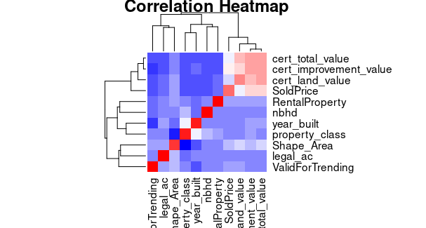
Multiple linear regression using R for the Real estate data set

sapply is used to check the data type of each column in the data frame and retain only the numeric columns. The resulting numeric_columns data frame will include all numeric columns from your original data frame your_data.

A heatmap is ploted to visualize the correlation between different numeric attributes in our dataset. This is useful for understanding how variables are related to each other.

R

# Assuming 'ConveyanceDate' is a date-time attribute
library(forecast)
decomposition <- stl(ts(data$SoldPrice, frequency = 12),
                     s.window = "periodic")
plot(decomposition)

Output:

Multiple linear regression using R for the Real estate data set

The code decomposes a time series of ‘SoldPrice’ using the ‘forecast’ package. It separates the time series into three components: trend, seasonality, and residuals, and then visualizes these components in four plots. This helps analyze trends and seasonal patterns in the ‘SoldPrice’ data and identifies irregularities or anomalies.

R

# Install the 'plotly' package for interactive 3D plots
library(plotly)

# Create a 3D scatter plot
plot_ly(data = data, x = ~year_built, y = ~SoldPrice, z = ~cert_total_value,
        color = ~property_class, type = 'scatter3d', mode = 'markers')

Output:

Multiple linear regression using R for the Real estate data set

The ‘plotly’ package to create an interactive 3D scatter plot. It visualizes a dataset called ‘df’ in three dimensions: ‘year_built’ on the x-axis, ‘SoldPrice’ on the y-axis, and ‘cert_total_value’ on the z-axis. Data points are colored according to the ‘property_class’ variable. The plot is interactive, allowing users to zoom, pan, and hover over data points for additional information, making it a powerful tool for exploring multidimensional patterns and relationships within the dataset.

Model building

Fit the multiple linear regression model using the lm function. Specify the dependent variable (in this case, the property price) and the independent variables (predictors, such as property size, number of bedrooms, number of bathrooms, and others). The model will estimate the coefficients for each predictor variable.

R

# Fit a multiple linear regression model using all columns except the response variable ('price')
model <- lm(SoldPrice ~ ., data = data)

# Display the summary of the linear regression model
summary(model)

Output:

 [ reached getOption("max.print") -- omitted 567 rows ]
---
Signif. codes:  0 ‘***’ 0.001 ‘**’ 0.01 ‘*’ 0.05 ‘.’ 0.1 ‘ ’ 1
Residual standard error: 97890 on 4649 degrees of freedom
Multiple R-squared:  0.9556,    Adjusted R-squared:  0.9487 
F-statistic: 138.1 on 725 and 4649 DF,  p-value: < 2.2e-16

Use the summary function to view the details of the regression model. This summary will provide information about the coefficients, standard errors, t-statistics, p-values, and the R-squared value, which indicates the goodness of fit.

Assess the quality of the model by examining the coefficients and their significance. A low p-value for a coefficient suggests it has a significant impact on the dependent variable. Also, consider the overall R-squared value, which indicates the proportion of variance in the dependent variable explained by the model.

Conclusion

Multiple Linear Regression is a powerful technique for real estate analysis, allowing you to understand how various factors contribute to property prices and make predictions based on those factors. It’s important to interpret the results carefully and validate the model to ensure its accuracy and reliability for making predictions.