Normal Distribution in Business Statistics

What is Normal Distribution?

Normal Distribution is defined as the probability distribution that tends to be symmetric about the mean; i.e., data near the mean occurs more as compared to the data far away from the mean. The two parameters of normal distribution are mean (μ) and standard deviation (σ). Hence, the notation of the normal distribution is

X ~ N (μ,σ²)

Probability Density Function (PDF) of Normal Distribution

The Probability Density Function (PDF) of a normal distribution, often denoted as f(x), describes the likelihood of a random variable taking on a specific value within the distribution. In simpler terms, it tells the probability of getting a particular result. For a normal distribution, the PDF is represented by the well-known bell-shaped curve. This curve is centered at the mean (average) value, and its shape is determined by the standard deviation, which measures how spread out the data is. The PDF shows that values near the mean are more probable, while values farther from the mean are less likely.

The PDF of a normal distribution is defined by:

, -∞ < x < ∞

Where,

• f(x) represents the probability density at a specific value x.
• μ is the mean, which indicates the center or average value of the distribution.
• σ is the standard deviation, which measures how spread out the data is.
• π is approximately 3.1416, a mathematical constant.
• e is the mathematical constant, measured at approximately 2.7183.

Standard Normal Distribution

As different combinations of μ and σ lead to different normal distributions. The Standard normal distribution is defined as the value of normal distribution at μ = 0 and σ = 1. This is known as z-transformation.

Since Z is symmetrical about zero,

• P(Z < -z) = P(Z > z) = 1 – P(Z < z)
• P(Z > -z) = P(Z < z)

Example:

If X ~ (49, 64), calculate:

(i) P (X < 52)

(ii) P (X > 60)

(iii) P (X < 45)

(iv) P (|X – 49| < 5)

Solution:

(i) P (X < 52) = = P(Z < 0.375) = 0.6443

P (X < 52) = 0.6443

(ii) P (X > 60) = = P(Z > 1.375) = 1 – P(Z < 1.375) = 0.91466

P (X > 60) = 0.91466

(iii) P(X < 45) = = P(Z < -0.5) = 1 – P(Z < 0.5) = 0.69146

P(X < 45) = 0.69146

(iv) P (|X – 49| < 5) = P ( -5 < (X – 49) < 5)

= P (44 < X < 54)

= P (X < 54) – P (X < 44)

= 

= P (Z < 0.625) – P(Z < -0.625)

= P(Z < 0.625) – [ 1 – P(Z < 0.625)]

= 0.73401 – (1 – 0.73401)

P (|X – 49| < 5) = 0.46802

Properties of Normal Distribution

1. Equality of Mean, Median, and Mode: In a normal distribution, the average (mean), middle value (median), and most frequent value (mode) are all the same.
2. Positive Value: For any value of x, f(x) will have a positive value.
3. Defined by Mean and Standard Deviation: A normal distribution is uniquely determined by two parameters, the average (mean) and the spread or variability (standard deviation). These parameters describe its uni-modal, bell-shaped, and symmetrical curve.
4. Symmetry at the Center: A normal distribution curve is symmetrical. If you fold it in half at the center, both sides look the same. This means that the values on one side of the mean are like a mirror image of the other side.
5. Total Area under the Curve: The entire area under the normal distribution curve adds up to 1. In simpler terms, if you add up all the probabilities of all possible values, it equals 100%.
6. Half of Values on each side of the Center: Exactly half of the values are to the right of the center, and the other half is to the left of the center. This reflects the even distribution of data.
7. One Peak: The normal distribution curve has only one hump or peak. It does not have multiple peaks. This is called a uni-modal distribution.

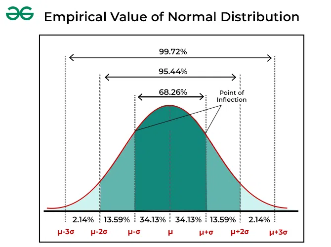
The Empirical Rule

In most cases with normal distributions, about 68.27% of the data will be found within one standard deviation above or below the average. Approximately 95.45% of the data falls within two times the standard deviation range, and around 99.73% falls within three times the standard deviation range. This is often called the “Empirical Rule,” which helps us understand where the majority of data in a normal distribution is located.

In other words, μ ± 1σ covers 68.27% of the area, μ ± 2σ covers 95.45% of the area, and μ ± 3σ represents 99.73% of the area.

Parameters of Normal Distribution

The parameters of the Normal Distribution, also known as the Gaussian Distribution, are the mean and the standard deviation. The mean represents the average or central value of the data, while the standard deviation measures the spread or variability of the data points. Together, these parameters describe the shape and characteristics of the bell-shaped curve that is typical of the Normal Distribution. The mean determines the center of the curve, and the standard deviation controls how wide or narrow it is. These parameters are essential for understanding and analysing data in various fields, including statistics, science, and finance.

I. Mean of Normal Distribution

In a normal distribution, the mean represents the central value where most data clusters. It determines the peak of the bell-shaped curve on a graph. If you change the mean, the whole curve shifts left or right on the horizontal axis. Essentially, the mean is the average value in the dataset, indicating where the data tends to center around, and it is a key factor for understanding the central tendency of the data. The mean in a normal distribution is denoted by the symbol μ (mu).

II. Standard Deviation of Normal Distribution

The normal distribution typically has a positive standard deviation. The mean indicates where the graph is balanced, while the standard deviation shows how much the data is spread out. A smaller standard deviation means the data is closer together, resulting in a narrower graph. Conversely, a larger standard deviation means the data is more spread out, resulting in a wider graph. Standard deviations help divide the area under the normal curve, with each division representing a percentage of data within a particular part of the graph. The formula for the standard deviation (σ) in a normal distribution is given as follows:

σ = √Variance = √σ²

Where,

• σ represents the standard deviation.
• σ² represents the variance.
• X represents individual data points.
• μ represents the mean (average) of the data.
• N represents the total number of data points.

Curve of Normal Distribution

The curve of a normal distribution, often referred to as a bell curve, is a symmetrical, smooth, and continuous graph that depicts the distribution of data. It has the following characteristics:

1. Symmetry: The curve is perfectly symmetrical around its center, which is the mean (average) value. This means that if you were to fold the curve in half at the mean, both sides would match like a mirror image.

2. Bell Shape: The curve takes the form of a bell, with a single peak at the mean. It rises to the peak, gradually descends on both sides and extends infinitely in both directions.

3. Mean as the Peak: The highest point of the curve is precisely at the mean value. This signifies that the mean is the most likely outcome in the distribution.

4. Standard Deviation Controls Spread: The spread or width of the curve is determined by the standard deviation. A smaller standard deviation results in a narrower, taller curve, while a larger standard deviation leads to a wider, shorter curve.

5. Tail Ends: As the curve moves away from the mean, it gets closer to the horizontal axis but never touches it. This means that there is always some probability of extreme values, although they become increasingly rare as you move further from the mean.

Examples of Normal Distribution

Example 1:

If the value of a random variable is 8, the mean is 10, and the standard deviation is 3, then find the probability density function (PDF) of the normal distribution at this value.

Solution:

To find the PDF at the value of the random variable (8), use the formula for the normal distribution.

According to the given information, we have, Mean (μ) = 10, Standard Deviation (σ) = 3, and e is the base of the natural logarithm (approximately 2.71828)

Now, putting the values in the formula, we get:

f(8) = 0.10648

Example 2:

If the value of a random variable is 12, the mean is 15, and the standard deviation is 2, then find the probability density function (PDF) of the Gaussian distribution at this value.

Solution:

To find the PDF at the value of the random variable (12), use the formula for the normal distribution,

According to the given information, we have, Mean (μ) = 15, Standard Deviation (σ) = 2, and e is the base of the natural logarithm (approximately 2.71828)

Now, putting the values in the formula, we get,

f(12) = 0.06475

Applications of Normal Distribution in Business Statistics

Normal Distribution is used in business statistics in the following ways:

1. Quality Control: Companies use the normal distribution to monitor and maintain the quality of their products. By analysing measurements and defects, they can assess if the production process is within acceptable limits.

2. Market Research: In market research, the normal distribution helps analyse customer preferences, buying patterns, and survey data. This aids in making informed marketing and product development decisions.

3. Financial Analysis: Financial analysts use the normal distribution to model and predict stock prices, asset returns, and investment risks. It’s the foundation for tools like the Black-Scholes model for options pricing.

4. Performance Evaluation: HR departments use the normal distribution to evaluate employee performance. It can help determine salary structures and performance bonuses, and identify underperforming or exceptional employees.

5. Supply Chain Management: Normal distribution assists in optimising inventory levels, demand forecasting, and managing production processes to ensure products are available when needed.

6. Risk Assessment: Businesses assess various risks, including credit risk, market risk, and operational risk, using the normal distribution to quantify and manage these risks effectively.

7. Credit Scoring: Financial institutions use the normal distribution to build credit scoring models, determining an individual’s creditworthiness and loan approval.