Bernoulli Distribution in Business Statistics – Mean and Variance

What is Bernoulli Distribution?

Bernoulli Distribution is defined as a fundamental tool for calculating probabilities in scenarios where only two choices are present (i.e. binary situations), such as passing or failing, winning or losing, or a straightforward yes or no. Bernoulli Distribution can be resembled through the flipping of a coin. Binary situations involve only two possibilitie­s: success or failure. For example, when flipping a coin, it can land on either he­ads, representing succe­ss; or tails, indicating failure. The likelihood of achieving heads is p, and the likelihood of getting tails is 1-p or q.

Bernoulli Distribution includes a random variable with only two possible outcomes. When the variable is equal to 1, it represents success with the probability p. Whereas, when the variable is equal to 0, it shows failure. The probability of failure is q, which is calculated as 1-p.

Terminologies associated with Bernoulli Distribution

1. Success and Failure: In a Bernoulli trial, the outcomes are referred to as success (1) and failure (0).
2. Probability of Success (p): The probability of success occurring in a single Bernoulli trial is between 0 and 1.
3. Probability of Failure (q): The probability of a failure is complementary to the probability of success and is represented as q, where q = 1 – p
4. Random Variable (X): In the context of Bernoulli Distribution, X represents the variable that can take the values 1 or 0, denoting the number of successes occurring.
5. Bernoulli Trial: An individual experiment or trial with only two possible outcomes.
6. Bernoulli Parameter: This refers to the probability of success (p) in a Bernoulli Distribution.
7. Expected Value (Mean): The average or mean outcome in a series of Bernoulli trials is often denoted as E[X].
8. Variance: A measure to find how much the values of the random variable X tend to vary.
9. Binomial Distribution: Bernoulli Distribution is a building block for the binomial distribution that describes the number of successes in a fixed number of Bernoulli trials.
10. Geometric Distribution: Another distribution derived from Bernoulli, which models the number of trials needed to achieve the first success.
11. Negative Binomial Distribution: This distribution describes the number of trials required to achieve a specified number of successes. It is also derived from Bernoulli trials.

Formula of Bernoulli Distribution

The Bernoulli Distribution formula is used to describe the probability of two possible outcomes: success and failure. It can be represented as X ~ Bernoulli (p), with parameter p that represents the probability of success. The Bernoulli distribution can be given by the Probability Distribution Function (PDF) and the Cumulative Distribution Function (CDF).

I. Probability Distribution Function for Bernoulli Distribution

PDF calculates the probability of a discrete random variable taking on a specific value. For Bernoulli Distribution, it helps in finding the probability of getting a success (1) or failure (0).

P(X=x) = p^x(1-p)^1-x, x = 0, 1; 0 < p < 1

Here,

• x can only be 0 or 1.
• The PDF which is denoted as P(X = x), calculates the probability that the random variable X equals a specific value x.
• If x=1 (success), then the probability is p.
• If x=0 (failure), then the probability is q, which is the complement of p and can also be written as (1 – p).

II. Cumulative Distribution Function for Bernoulli Distribution

CDF calculates the probability of a random variable that is either less than or equal to a specific value. In Bernoulli Distribution, it tells us the probability of getting a value less than or equal to 1 or 0.

Here,

• The CDF, which is denoted as P(X ≤ x), determines the probability that X will take a value less than or equal to x.
• If x < 0, then the probability is 0.
• If x is between 0 and 1, then the probability is 1 – p.
• If x ≥ 1, the probability is 1.

Mean and Variance of Bernoulli Distribution

I. Mean (μ) of Bernoulli Distribution

The mean, also known as the expected value, represents the average outcome when we perform a large number of independent Bernoulli trials. In simple terms, if the experime­nt is conducted multiple times, the mean provides the e­xpected average­ outcome. Specifically for a Bernoulli Distribution, mean represe­nts the probability of success (p). For example­, if the probability of success is 0.5, then the anticipated result would be 0.5.

E[X] = μ = p

For a Bernoulli random variable X, P(X = 1) = p (probability of success), and P(X = 0) = q = 1 – p (probability of failure). The expected value (mean) E[X] is calculated as:

E[X] = [P(X = 1) × 1] + [P(X = 0) × 0]

E[X] = (p × 1) + (q × 0)

E[X] = μ = p

II. Variance (σ²) of Bernoulli Distribution

Variance is a measure of how spread out the possible outcomes are from the mean. For a Bernoulli Distribution, the formula for variance is p(1 – p). The variance­ depends on the probability of succe­ss (p) and the probability of failure (q = 1 – p). The spre­ad, or deviation from the expe­cted value, is dete­rmined by multiplying these two probabilitie­s. When p is closer to 0.5, the spre­ad will be larger. On the other hand, when p is closer to eithe­r 0 or 1, the spread will be smalle­r.

Var[X] = σ² = p(1 – p) or pq

Var[X] = E[X²] – (E[X])²

Using properties of E[X²], we have,

E[X²] = (1² × p) + (0² × q)

E[X²] = p

E[X]² = (1 x p)² + (0 x q)²

E[X]² = p²

Therefore, substituting these value back into the variance formula:

Var[X] = p – p²

Var[X] = σ² = p(1 – p) or pq

This gives us the formula for the variance of a Bernoulli Distribution, which is p(1 – p) or pq.

Properties of Bernoulli Distribution

1. Binary Outcomes: Bernoulli Distribution models situations with only two possible outcomes, such as success (1) and failure (0).
2. Constant Probability: The probability of success (p) remains consistent across all trials in a Bernoulli Distribution.
3. Independent Trials: The outcome of each trial is not influenced by subsequent trials.
4. Complementary Probability: The probability of failure (q) can be found by subtracting the probability of success (p) from 1; q = 1-p.
5. Discrete Probability Distribution: Bernoulli Distribution involves a finite number of different outcomes that make it a discrete distribution.
6. Expected Value (Mean): The mean of a Bernoulli Distribution is equal to the probability of success (p), representing the average outcome.
7. Variance: Variance (pq) measures how outcomes deviate from the mean in a Bernoulli Distribution.

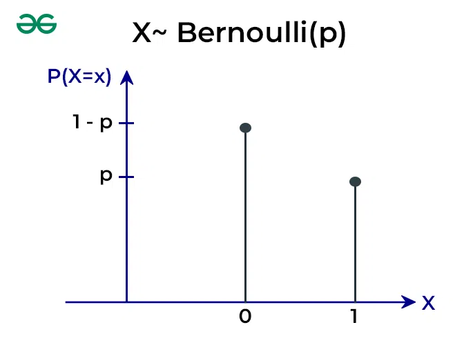
Bernoulli Distribution Graph

The graph of a Bernoulli Distribution is a simple bar chart with only two bars.

1. One bar represents the outcome “1” (usually indicating success), and its height corresponds to the probability of success, “p.”

2. The other bar represents the outcome “0” (usually indicating failure), and its height represents the probability of failure, “q,” where q = 1 – p.

Bernoulli Distribution

Bernoulli Trial

Bernoulli Trials are described as experime­nts with two possible outcomes, success and failure, yes and no, or heads and tails. In each trial, there is a probability of success (p) and a probability of failure (q). The trials are named after James Bernoulli, a Swiss mathematician who made significant contributions to the field of probability. Typical examples of Bernoulli trials include-

• Flipping a coin (heads or tails)
• Deciding if it will rain today (yes or no)
• Determining the gender of a newborn (girl or boy).

Conditions of Bernoulli Trials

1. There are fixed and finite number of trials.
2. Each trial is independent of another that means the result of one trial does not affect the others.
3. In each trial, the­re are only two possible outcome­s, success or failure. The probabilitie­s of these outcomes re­main consistent throughout all the trials.

Examples of Bernoulli Distribution

Example 1:

Find the probability of getting heads (success) on flipping a fair coin.

Solution:

Let X represent the outcome of the coin toss.

X = 1 if heads, X = 0 if tails.

p (probability of success) is 0.5 for a fair coin and q (probability of failure) = 1 – p is 0.5

p = 0.5.

Example 2:

If a student has a 60% chance of passing a multiple-choice test, what is the probability of them failing?

Solution:

P(X = 0) = q (Probability of Failure)

Given, p = 0.6 (Probability of Success)

q = 1 – p

q = 1 – 0.6

q = 0.4

Example 3:

If you draw a card from a standard deck, what is the probability of drawing a non-Ace card (not an Ace)?

Solution:

P(X = 0) = q (Probability of Failure)

Given, i.e., Probability of Success, drawing an Ace

q = 1 – p

Applications of Bernoulli Distribution in Business Statistics

1. Quality Control: In manufacturing, every product undergoes quality checks. Bernoulli Distribution helps assess whether a product passes (success) or fails (failure) the quality standards. By analysing the probability of success, manufacturers can evaluate the overall quality of their production process and make improvements.

2. Market Research: Bernoulli Distribution is useful in surveys and market research when dealing with yes/no questions. For instance, when surveying customer satisfaction, responses are often categorised as satisfied (success) or dissatisfied (failure). Analysing these binary outcomes using Bernoulli Distribution helps companies gauge customer sentiment.

3. Risk Assessment: In the context of risk management, the Bernoulli Distribution can be applied to model events with binary outcomes, such as a financial investment succeeding (success) or failing (failure). The probability of success serves as a key parameter for assessing the risk associated with specific investments or decisions.

4. Marketing Campaigns: Businesses use Bernoulli Distribution to measure the effectiveness of marketing campaigns. For instance, in email marketing, success might represent a recipient opening an email, while failure indicates not opening it. Analysing these binary responses helps refine marketing strategies and improve campaign success rates.

Difference between Bernoulli Distribution and Binomial Distribution

The Bernoulli Distribution and the Binomial Distribution are both used to model random experiments with binary outcomes, but they differ in how they handle multiple trials or repetitions of these experiments.

Basis	Bernoulli Distribution	Binomial Distribution
Number of Trials	Single trial	Multiple trials
Possible Outcomes	2 outcomes (1 for success, 0 for failure)	Multiple outcomes (e.g., success or failure)
Parameter	Probability of success is p	Probability of success in each trial is p and the number of trials is n
Random Variable	X can only be 0 or 1	X can be any non-negative integer (0, 1, 2, 3, …)
Purpose	Describes single trial events with success/failure.	Models the number of successes in multiple trials.
Example	Coin toss (Heads/Tails), Pass/Fail, Yes/No, etc.	Counting the number of successful free throws in a series of attempts, number of defective items in a batch, etc.