Binomial Distribution in Business Statistics – Definition, Formula & Examples

What is Binomial Distribution?

Binomial Distribution is a probability distribution that models the number of successes in a fixed number of independent, identical trials, where each trial can result in one of two outcomes, success or failure. It is often used to analyse and predict the probability of success or failure in situations with binary outcomes, such as whether a product will be defective or not, whether a customer will make a purchase or not, or whether a project will meet a deadline or not. In case, X is distributed binomially with parameters n and p, then X ~ Bin (n,p).

Key characteristics of Binomial Distribution:

• The number of trials is predetermined and remains constant.
• Each trial is independent of the others, meaning the outcome of one trial does not affect the outcome of subsequent trials.
• The probability of success, p, remains the same.
• Each trial results in one of two possible outcomes, typically denoted as success (S) and failure (F).

Formula of Binomial Distribution

For any variable X, binomial distribution formula can be written as:

P(X = x) = ⁿC_x p^x (q)^n-x, x = 0, 1, 2,……,n; 0 < p < 1

Where, 

P(X=x) represents the probability of getting x successes in n experiments,

ⁿC_x is the binomial coefficient and is equal to

p is the probability of success in a single experiment.

q is the probability of failure in a single experiment, and q = 1 – p

n is the total number of experiments.

Properties of Binomial Distribution

1. Binomial distribution has a fixed number of independent trials; i.e., n.
2. In each trial, there are only two outcomes, success or failure.
3. The probability of success (p) remains constant across all trials.
4. Each trial is independent, with no impact on others.
5. It is a discrete probability distribution with specific, countable values.
6. Probability Distribution Function (PDF) calculates probabilities for ‘x’ successes in ‘n’ trials.
7. Mean (μ) equals np, and Variance (σ²) equals npq.
8. The shape of the binomial curve varies based on ‘n’ and ‘p,’ tending towards symmetry with larger ‘n.’
9. For large ‘n,’ it approximates a normal distribution (Central Limit Theorem).
10. Cumulative Distribution Function (CDF) finds cumulative probabilities for ≤ ‘x’ successes.

Negative Binomial Distribution

In probability and statistics, the negative binomial distribution is used in tracking the number of trials required to get r^th success. The PDF of negative binomial distribution is,

 P(X = x) = ^x-1C_r-1 p^r q^x-r, x = r, r+1, ……..; 0 < p < 1

For instance,

1. Think of a basketball player attempting to make baskets. Consider each successful basket as a success and any missed shot as a failure. The negative binomial distribution then tells the number of failed shots made before getting a successful basket.

2. Imagine a student taking a pop quiz, where every correct answer is a success, and every wrong answer is a failure. The negative binomial distribution helps determine how many failed answers he gives before giving a right answer.

Mean and Variance of Binomial Distribution

Mean (μ): The mean represents the average number of successes in a binomial distribution. It is calculated by multiplying the number of trials (n) by the probability of success (p). To find the mean, simply multiply the number of trials (how many times you are repeating the experiment) by the probability of a successful outcome in each trial. This will give the expected or average number of successes.

μ = np

Variance (σ²): The variance measures how much the number of successes varies from the mean in a binomial distribution. It is calculated by multiplying the number of trials (n) by the probability of success (p) and the probability of failure (q, where q = 1 – p). To find the variance, calculate the probability of failure (q) by subtracting the probability of success (p) from 1. Then, multiply the number of trials (n) by both p and q. This will give a measure of how spread out or variable the number of successes is in the distribution.

σ² = npq

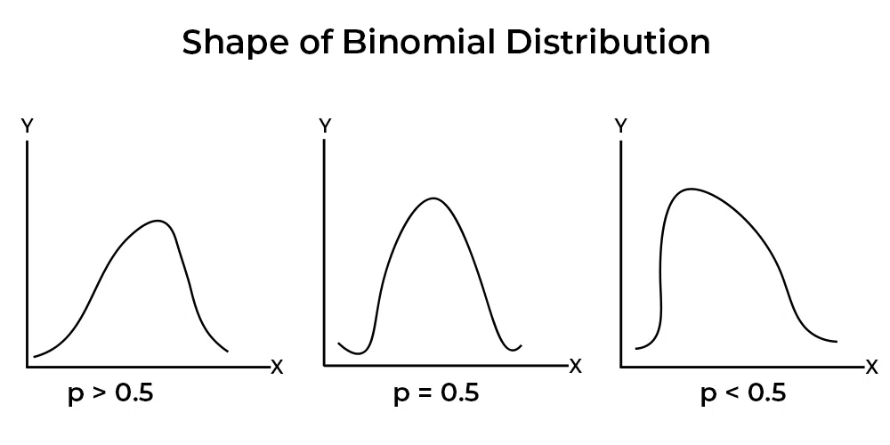
Shape of Binomial Distribution

Binomial Distribution may be symmetrical or skewed. If the probability of sucess, p, is equal to 0.5, then the binomial distribution would be symmetrical, regardless of the value of n. If p < 0.5, the distribution will be positively skewed; while for p > 0.5, the distribution will be negatively skewed. Further, for a given value of n, the greater is the departure from 0.5, the greater is the degree of skewness.

Solved Examples of Binomial Distribution

Example 1:

If a biased coin that lands on heads with a probability of 0.6, is flipped 4 times, what is the probability of getting exactly 2 heads?

Solution:

Here, Number of trials (n) = 4

Probability of getting a head (p) = 0.6

Probability of getting a tail (q) = 1 – p = 1 – 0.6 = 0.4

Using the binomial distribution formula:

P(X = x) = ⁿC_x p^x (q)^n-x

P(X = 2) = ⁴C₂ × (0.6)² × (0.4)^4-2

P(X = 2) = 6 × 0.36 × 0.16

P(X = 2) = 0.3456

Thus, The probability of getting exactly 2 heads in 4 coin flips is 0.3456.

Example 2:

In a multiple-choice quiz, each question has 4 options. On randomly guessing the answers to 8 questions, what is the probability of getting at least 6 correct?

Solution:

Here, Number of trials (n) = 8

According to question, we need to find, P( X ≥ 6) = P(X = 6) + P(X = 7) + P(X = 8)

Using the binomial distribution formula,

P(X = 6) =28 × 0.00024414 × 0.5625

P(X = 6) = 0.0038

P(X = 7) = 8 × 0.000061035 × 0.75

P(X = 7) = 0.00036

P(X = 8) = 1 x 0.0000152588 x 1

P(X = 8) = 0.000015

Adding these probabilities together

P(X ≥ 6) = 0.0038 + 0.00036 + 0.000015

P(X ≥ 6) = 0.004175

Hence, The probability of getting at least 6 correct answers when randomly guessing on 8 questions is approximately 0.004175.

Uses of Binomial Distribution in Business Statistics

In business, binomial distribution is used for the following reasons:

1. Quality Control: Quality control is crucial in any business to ensure that products meet specific standards and have minimal defects. The binomial distribution can be used to assess product quality and defect rates by calculating the probability of having a certain number of defective items in a batch. For instance, in a toy-making factory, in order to check how many toys have the problem of missing parts.

2. Conversion Rates: Conversion rates are an important aspect of the sales and marketing department, as every business wants to know how likely a customer is to purchase a product or sign up for their newsletter. The binomial distribution helps in analysing customer conversion by estimating the probability of a specific number of conversions from a given number of interactions, such as website visits or email opens.

3. Credit Risk: Financial institutions use the binomial distribution to evaluate credit risk. When a bank lends money, they want to know how likely it is for people to not pay it back. By assessing the probability of loan defaults, lenders can make better decisions about lending money and determine the terms and interest rates associated with loans.

4. Inventory Management: Inventory management is about making sure that a business maintains a sufficient level of stock to fulfill demand without overstocking or running out of products. The binomial distribution can be helpful in predicting stock shortages or surpluses by calculating the probability of a certain level of demand over a specified time period.

5. Employee Attrition: Employee turnover is a concern for many businesses, as hiring new employees is a cost to the company. The binomial distribution is a helpful tool for companies in knowing employee attrition by estimating the probability of a certain number of employees leaving the organisation within a given time period. This information can guide human resource planning and retention strategies.

6. Market Research: When a company does surveys to find out the likes and dislikes of people. The binomial method helps them understand how likely it is for a specific number of people to give particular answers.

7. Project Management: While managing a project, it is important to know how likely it is to succeed or fail. The binomial method can help by estimating the chances of success based on past experiences.

8. Risk Analysis: Businesses face various risks, such as market volatility, supply chain disruptions, and legal challenges. The binomial distribution can be used in risk analysis to assess and mitigate these risks. By calculating the probabilities of different risk scenarios, businesses can develop risk management strategies to protect their interests and assets.

Real-Life Scenarios of Binomial Distribution

Some real-life scenarios where binomial distribution is used are:

1. Material Usage in Manufacturing: In manufacturing, predict the quantity of raw materials used (success) versus the amount that remains unused (failure) in the production process. Binomial distribution aids in cost management. Conducting surveys to gather positive and negative reviews from the public regarding specific products or places.

2. TV Channel TRP: Using “YES” or “NO” surveys to assess the viewership of a particular TV channel among people.

3. Workplace Gender Demographics: Estimating the gender distribution of employees within an organisation.

4. Election Votes: Counting the total votes received by an electoral candidate based on a binary system, where each voter’s choice is represented as 1 when people vote for the candidate or 0 if people do not vote for the candidate.

Difference Between Binomial Distribution and Normal Distribution

Basis	Binomial Distribution	Normal Distribution
Type of Distribution	Discrete	Continuous
Events	Finite and countable	Infinite and uncountable
Probability Calculation	Uses specific probabilities for each outcome	Uses a probability density function
Shape	Can be skewed or symmetric (depends on parameters)	Always symmetrical (bell-shaped)
Influence of Sample Size	Significantly impacts the shape	Less influenced by sample size
Approximation	Approaches normal distribution with a large sample size	Always has a normal distribution shape