Multivariate Analysis in R

Analyzing data sets with numerous variables is a crucial statistical technique known as multivariate analysis. Many different multivariate analysis procedures can be carried out using the well-liked programming language R. A number of libraries and functions are available in the well-liked programming language R for carrying out multivariate analysis. In this post, we’ll go through various functions and methods for implementing multivariate analysis in R Programming Language.

• Multivariate analysis: The statistical analysis of data sets with several variables is referred to as multivariate analysis. In order to comprehend the underlying structure of the data and to find patterns and interactions between variables, multivariate analysis is performed.
• Multivariate data: Data sets with multiple variables are referred to as multivariate data. Multivariate data can be quantitative or categorical, and it is possible to analyze it using a number of different statistical methods.
• Dimensionality reduction: Dimensionality reduction is the technique of minimizing information loss while minimizing the number of variables in a data set. Multivariate analysis frequently uses dimensionality reduction to streamline the data and make it simpler to analyze.
• Exploratory and confirmatory analysis: Without having any preconceived notions, exploratory analysis is used to examine and comprehend the dataset. A specific hypothesis is validated through confirmatory analysis.

Data cleaning and transformation

Loading the data into R is the initial step in performing multivariate analysis in R. The data can be in a variety of formats, including.csv , .txt, and .xls. The data must next be cleaned and changed into an analysis-ready format. At this step, the data is cleaned up, scaled, and otherwise transformed as necessary.

Multivariate Analysis Technique

On the basis of the study question and data set, the following step is to select an appropriate multivariate analysis technique. Multivariate analysis can be done using R using a variety of tools and packages. Some of the multivariate analysis methods in R that are most frequently used are as follows:

• Principal Component Analysis (PCA) – Using a new collection of uncorrelated variables termed principal components, PCA is a technique for reducing the dimensionality of a dataset. With the help of this method, you may narrow down the dataset’s most crucial variables and see the information in a smaller dimension.
• Factor Analysis (FA) – Finding the underlying causes of the correlation between observable variables is done using the Factor Analysis approach. Latent variables that could be challenging to measure directly are found using this technique.
• Cluster Analysis – A method for finding patterns or clusters within a dataset is cluster analysis. Based on their similarity across several variables, it is used to group related observations together.
• Discriminant Analysis – Discriminant analysis is a method for determining how groups differ from one another based on a variety of factors. It is used to identify the factors that influence group differences the most.
• Canonical Correlation Analysis (CCA)- CCA is a method for figuring out the relationship between two sets of variables. It is employed to determine the connection between variables in two various datasets.
• Multidimensional Scaling (MDS)- The similarity or dissimilarity between observations in a high-dimensional dataset can be seen using the MDS approach. It is used to make the data less complex and to see it on a smaller scale.
• Correspondence Analysis (CA)- Analyzing the association between categorical variables is done using the CA approach. The connections between the categories of two or more categorical variables are found using this method.

These are some of the multivariate analysis methods most frequently used in R, and each one has pros and cons based on the research issue and the type of data being analyzed. Using the built-in iris data set in R, the following example shows how to perform PCA on a data set:

R

# Load the iris data set
data(iris)

# Select the variables to include
# in the PCA analysis
vars <- c("Sepal.Length", "Sepal.Width",
          "Petal.Length", "Petal.Width")

# Subset the data to include
# only the selected variables
data_subset <- iris[, vars]

# Scale the data
data_scaled <- scale(data_subset)

# Perform PCA
pca <- prcomp(data_scaled,
              center = TRUE, scale. = TRUE)

# Print the summary of the PCA results
summary(pca)

Output:

Importance of components:
                          PC1    PC2     PC3     PC4
Standard deviation     1.7084 0.9560 0.38309 0.14393
Proportion of Variance 0.7296 0.2285 0.03669 0.00518
Cumulative Proportion  0.7296 0.9581 0.99482 1.00000

The results of the PCA are summarized in this output, which also includes the standard deviation, variance proportion, and cumulative proportion for each principal component. The first principal component accounts for 72.96 percent of the total variation in the data, whereas the second and third components each account for 22.8 percent and 3.6 percent of the variance. The data may be efficiently reduced to three dimensions because the cumulative proportion reveals that the first three components account for more than 99% of the overall variance in the data.

Different Visualizations for the dataset

We can better comprehend the connections between the variables and spot any patterns or trends by visualizing the data. To construct several plot types in R, including scatter plots, box plots, and histograms, we can use a number of libraries.

R

# Load the ggplot2 library
library(ggplot2)

# Generate some sample data
data <- data.frame(
  var1 = rnorm(100),
  var2 = rnorm(100),
  group = sample(1:4, 100, replace = TRUE)
)

# Create a scatter plot
ggplot(data, aes(x = var1, y = var2)) +
  geom_point()

Output:

R

# Create a box plot
ggplot(data, aes(x = factor(group), y = var1)) +
  geom_boxplot()

Output:

R

# Create a histogram
ggplot(data, aes(x = var1)) +
  geom_histogram()

Output:

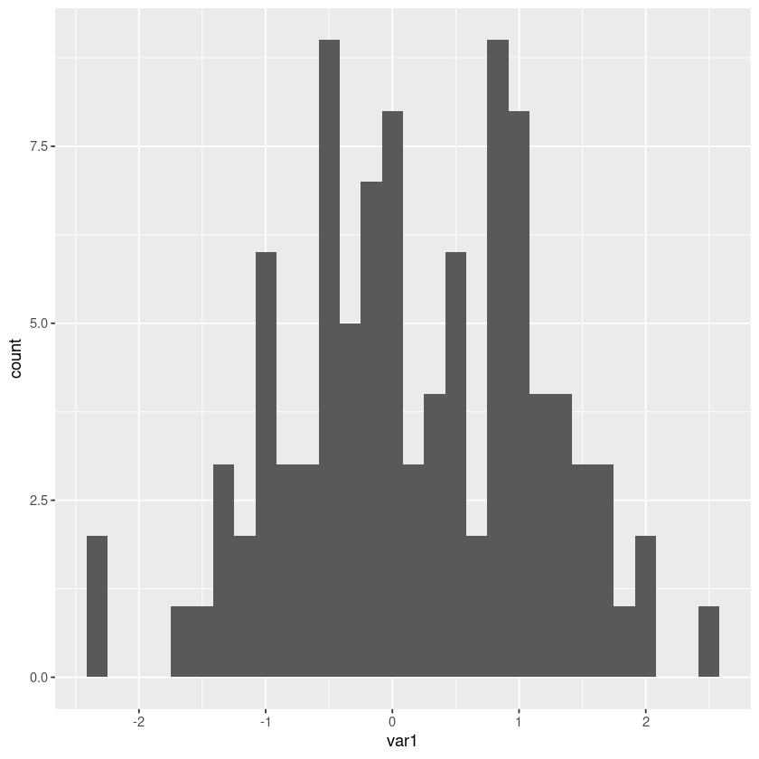
Histogram using ggplot2

A correlation matrix plot can also be made using the corrplot() method from the corrplot package.

R

# Load the corrplot library
library(corrplot)

# Create a correlation matrix plot
corrplot(cor(data), method = "circle")

Output:

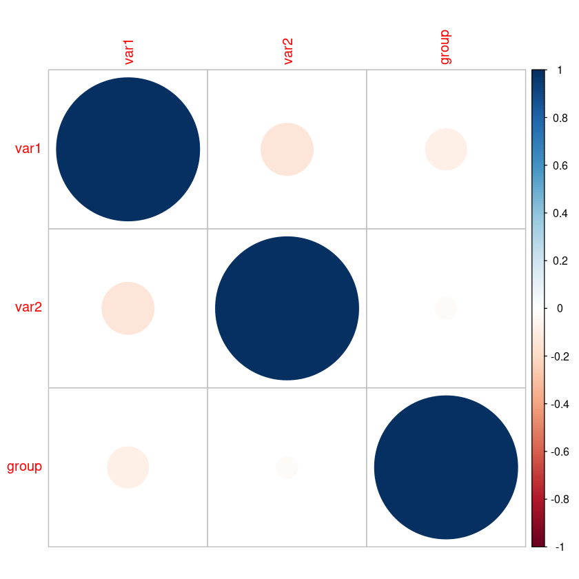
Correlation plot using corrplot package in R

Descriptive Statistical Measures

In multivariate analysis, variance, covariance, and correlation are crucial measurements because they allow us to comprehend the connections between the variables. Many functions in R can be used to compute these metrics.

R

# Calculate the variance
var(data$var1)

# Calculate the covariance
cov(data$var1, data$var2)

# Calculate the correlation
cor(data$var1, data$var2)

Output:

0.964993019401173
-0.131206113335423
-0.133108806509815

The psych library can also be used to compute various metrics including skewness, kurtosis, and factor analysis.

R

# Load the moments package
library(moments)

# Load the psych library
library(psych)

# Calculate the skewness
skewness(data$var1)

# Calculate the kurtosis
kurtosis(data$var1)

# Perform factor analysis
fa(data)

Output:

-0.113671043634579
2.58907790883746

R

# Perform factor analysis
fa(data)

Output:

Factor Analysis using method =  minres
Call: fa(r = data)
Standardized loadings (pattern matrix) based upon correlation matrix
        MR1     h2     u2 com
var1   1.00 0.9957 0.0043   1
var2  -0.13 0.0171 0.9829   1
group -0.08 0.0062 0.9938   1

                MR1
SS loadings    1.02
Proportion Var 0.34

Mean item complexity =  1
Test of the hypothesis that 1 factor is sufficient.

df null model =  3  with the objective function =  0.03 with Chi Square =  2.53
df of  the model are 0  and the objective function was  0 

The root mean square of the residuals (RMSR) is  0.02 
The df corrected root mean square of the residuals is  NA 

The harmonic n.obs is  100 with the empirical chi square  0.23  with prob <  NA 
The total n.obs was  100  with Likelihood Chi Square =  0.12  with prob <  NA 

Tucker Lewis Index of factoring reliability =  Inf
Fit based upon off diagonal values = 0.95
Measures of factor score adequacy             
                                                   MR1
Correlation of (regression) scores with factors   1.00
Multiple R square of scores with factors          1.00
Minimum correlation of possible factor scores     0.99

PCA and LDA

Two well-liked methods for multivariate analysis are PCA (Principal Component Analysis) and LDA (Linear Discriminant Analysis). Dimensionality reduction is accomplished with PCA, and classification is accomplished with LDA. For PCA and LDA in R, respectively, we can use the lda() function from the MASS library and the prcomp() function from the stats package.

R

# Load the stats and MASS libraries
library(stats)
library(MASS)

# Perform PCA
pca <- prcomp(data[, 1:3])
summary(pca)

# Perform LDA
lda <- lda(group ~ var1 + var2, data = data)
summary(lda)

Output:

Importance of components:
                          PC1    PC2    PC3
Standard deviation     1.0946 1.0498 0.9119
Proportion of Variance 0.3826 0.3519 0.2655
Cumulative Proportion  0.3826 0.7345 1.0000
        Length Class  Mode     
prior   4      -none- numeric  
counts  4      -none- numeric  
means   8      -none- numeric  
scaling 4      -none- numeric  
lev     4      -none- character
svd     2      -none- numeric  
N       1      -none- numeric  
call    3      -none- call     
terms   3      terms  call     
xlevels 0      -none- list 

The prcomp() method returns the dataset’s major components, their variances, and the percentages of total variance they account for. The coefficients of the linear discriminants and their accompanying classification accuracies are provided by the lda() function.

Conclusion

We can evaluate data with several variables using the potent statistical technique known as multivariate analysis. Using a variety of functions and methods, we covered how to implement multivariate analysis in R in this post. We discussed descriptive statistics, data visualization, computations of variance, covariance, and correlations, as well as PCA and LDA, two well-liked methods. We can get insights into intricate datasets and come to fact-based conclusions by comprehending and putting these strategies to use.