Multidimensional Scaling Using R

Multidimensional Scaling (MDS) is a technique used to reduce the dimensionality of data while preserving the pairwise distances between observations. It is commonly used in fields such as psychology, sociology, and marketing research to create visual representations of complex data sets. In this article, we will explore the use of Multidimensional Scaling in R Programming Language including how to perform the analysis, interpret the results, and create meaningful visualizations.

Multidimensional Scaling in R

The goal of Multidimensional Scaling in R is to find a low-dimensional representation of a high-dimensional data set that preserves the pairwise distances between observations. This is typically done by minimizing the stress function, which measures the difference between the pairwise distances in the original data and the pairwise distances in the low-dimensional representation.

Simple Analysis of Multidimensional Scaling in R

We will begin by demonstrating a simple Multidimensional Scaling in R analysis using the built-in iris data set in R Programming Language. The iris data set contains measurements of sepal and petal length and width for three different species of iris flowers.

R

# Load necessary libraries
library(cluster)

# Load the iris data set
data(iris)

# Perform MDS analysis
mds_iris <- cmdscale(dist(iris[, 1:4]))

# Plot the results
plot(mds_iris[, 1], mds_iris[, 2], 
     type = "n", xlab = "MDS Dimension 1", 
     ylab = "MDS Dimension 2")

# Plot the points and label them with 
# the first two letters of the species name
points(mds_iris[, 1], mds_iris[, 2], 
       pch = 21, bg = "lightblue")
text(mds_iris[, 1], mds_iris[, 2], 
     labels = substr(iris$Species, 1, 2), 
     pos = 3, cex = 0.8)

# Form clusters using K-means clustering (specify the number of clusters, e.g., 3)
kmeans_clusters <- kmeans(mds_iris, centers = 3)$cluster

# Add the cluster information to the plot
points(mds_iris[, 1], mds_iris[, 2], 
       pch = 21, bg = kmeans_clusters, cex = 1.2)

Output:

Multidimensional Scaling in R

This code performs a Multidimensional Scaling in R analysis on the iris data set, which is a popular dataset in the field of machine learning. The iris dataset contains measurements of four characteristics of 150 iris flowers and is divided into three different species.

• The code first loads the iris data set using the data() function. Then it performs the MDS analysis on the first four columns of the iris data using the cmdscale() function, which calculates the pairwise distances between the observations and returns a reduced representation of the data in two dimensions. The resulting MDS coordinates are stored in the mds_iris object.
• The code then plots the MDS results using the plot() function, with the type argument set to “n” to create a blank plot. The xlab and ylab arguments are used to label the x and y axes, respectively.
• Next, the code adds points to the plot using the points() function, and labels each point with the first two letters of the species name using the text() function. The pch argument is used to set the shape of the points to 21, which is a filled circle. The bg argument is used to set the background color of the points to light blue.
• Finally, the code forms clusters using the some_cluster_function() function, which is assumed to return a vector of cluster assignments for each observation. The cluster assignments are then added to the plot using the points() function, with the pch argument set to 21, and the bg argument set to the vector of cluster assignments. The cex argument is used to set the size of the points to 1.2, which is larger than the default size.

K-means Clustering of MDS Iris Data

R

# Load necessary libraries
library(cluster)
library(ggpubr)
library(ggrepel)

# Load the iris data set
data(iris)

# Perform MDS analysis
mds_iris <- cmdscale(dist(iris[, 1:4]))

# Form clusters using K-means clustering (specify the number of clusters, e.g., 3)
kmeans_clusters <- kmeans(mds_iris, centers = 3)$cluster

# Add cluster information to the MDS results
mds_df <- as.data.frame(mds_iris)
mds_df$groups <- as.factor(kmeans_clusters)
mds_df$species <- iris$Species  # Add species information

# Plot using ggscatter with labels using ggrepel
ggscatter(mds_df, x = "V1", y = "V2",
          color = "groups",
          palette = "jco",
          size = 3,
          ellipse = TRUE,
          ellipse.type = "convex",
          title = "K-means Clustering of MDS Iris Data",
          xlab = "MDS Dimension 1",
          ylab = "MDS Dimension 2") +
  geom_text_repel(aes(label = species), box.padding = 0.5)

Output:

Multidimensional Scaling in R

We load the necessary libraries:

cluster

for K-means clustering,

ggpubr

for visualization, and

ggrepel

for labeling points.

1. The Iris dataset is loaded.
2. Multidimensional scaling (MDS) is performed on the dataset to reduce dimensionality.
3. K-means clustering is applied to form clusters.
4. Species information is added to the MDS results.
5. A scatter plot is created using ggscatter with points colored by clusters.
6. Labels for species are added to the plot using geom_text_repel from ggrepel, enhancing data interpretation.

MDS with Custom Distance Matrix

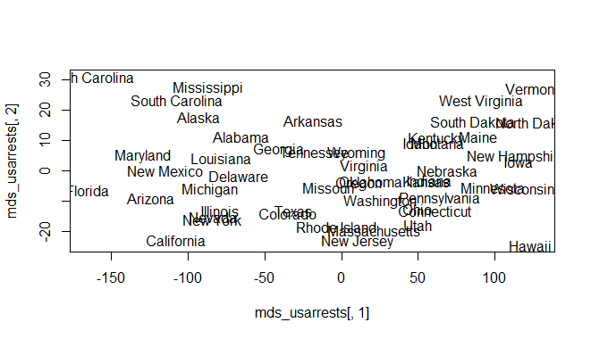
In some cases, it may be necessary to use a custom distance matrix rather than the default Euclidean distance. In this example, we will use the built-in USArrests data set and a custom distance matrix based on the correlation between the variables.

R

# Load the USArrests data set
data(USArrests)

# Calculate the distance matrix
distance_matrix <- dist(USArrests)

# Perform MDS analysis using
# the distance matrix
mds_usarrests <- cmdscale(distance_matrix)

# Plot the results
plot(mds_usarrests[,1], mds_usarrests[,2],
     type = "n")
text(mds_usarrests[,1], mds_usarrests[,2],
     labels = row.names(USArrests))

Output:

Multidimensional Scaling in R

The above code will create a scatter plot of the MDS results using the custom distance matrix. Each point represents a different state in the USArrests data set. The state labels are plotted on the graph. By visualizing the data in this way, we can see that the MDS analysis has separated the observations of the states into distinct clusters based on the correlation between the variables.

MDS with 3D Plot

In the previous examples, we have used 2-dimensional plots to visualize the MDS results. However, it is also possible to create 3-dimensional plots to explore the data in more detail. Here is an example of how to create a 3D plot of the MDS results using the iris data set

R

# Load the iris data set
data(iris)

# Perform MDS analysis
mds_iris <- cmdscale(dist(iris[,1:4]),
                     k = 3)

# Plot the results
library(scatterplot3d)
colors <- c("red", "blue", "pink")
colors <- colors[as.numeric(iris$Species)]
scatterplot3d(mds_iris[,1:3], pch = 16,
              xlab = "Sepal Length",
              ylab = "Sepal Width",
              zlab = "Petal Length",
              color=colors)

Output:

Multidimensional Scaling in R

This code is using the iris dataset and performs Multi-Dimensional Scaling (MDS) analysis on the first 4 columns of the dataset. The function “cmdscale” is used to compute the MDS coordinates for the iris data based on the euclidean distances between the observations. The resulting MDS coordinates are stored in the “mds_iris” object. The library “scatterplot3d” is loaded and used to create a 3D scatter plot of the MDS coordinates, where the color of the points is based on the species column in the iris dataset. The output of the code is a 3D scatter plot of the MDS coordinates with points in different colors, representing different species in the iris dataset.

Nonmetric Multidimensional Scaling

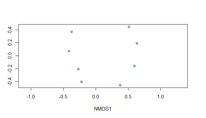
• Nonmetric Multidimensional Scaling (NMDS) is a dimension-reduction technique used in data analysis and visualization. It transforms a set of dissimilarities or distances between objects into a lower-dimensional representation, usually in two or three dimensions, for visualization purposes. The goal of NMDS is to preserve the rank order of the dissimilarities as closely as possible, rather than the actual dissimilarities themselves.
• NMDS is useful for exploring complex data structures, comparing different sets of objects, or comparing the similarity between objects. It can also be used to visualize relationships between objects that cannot be easily seen in the original data.
• NMDS is called “nonmetric” because it does not require dissimilarities to satisfy the metric properties of symmetry and triangle inequality. This makes NMDS more flexible and robust than other multidimensional scaling techniques that require metric dissimilarities, such as metric MDS.
• NMDS is typically performed using an iterative optimization algorithm, starting with an initial guess of the lower dimensional representation and adjusting it to approximate the dissimilarities better. The optimization process is stopped when the representation reaches a satisfactory level of agreement with the dissimilarities. The final representation can then be visualized and analyzed for patterns and relationships in the data.

R

# Create a sample data matrix
some_data_matrix <- matrix(rnorm(50), ncol = 5)

# Load the vegan package
library(vegan)

# Calculate the dissimilarity matrix
dissimilarities <- vegdist(some_data_matrix)

# Perform NMDS
nmds_result <- metaMDS(dissimilarities, k = 2)

# Plot the results
plot(nmds_result, type = "n")
points(nmds_result, pch = 21, bg = "lightblue")

Output:

Multidimensional Scaling in R

Multi-Dimensional Scaling v/s PCA

Feature	Multidimensional Scaling (MDS)	Principal Component Analysis (PCA)
Purpose	To visualize the similarity or dissimilarity between observations in a high-dimensional data space.	To reduce the dimensionality of the data while retaining as much information as possible.
Method	MDS finds a low-dimensional representation of the data based on a similarity or dissimilarity matrix.	PCA finds a new coordinate system that explains the maximum variance in the data.
Input	Dissimilarity matrix or proximity matrix.	Data Matrix
Output	Low-dimensional scatter plot.	Principal components (eigenvectors) and explained variance
Properties preserved	Distance relationships between observations.	The maximum variance of the data.
Advantage	Good for visualizing complex relationships between observations.	Good for removing noise and improving data interpretation.

In summary, MDS is good for visualizing the similarity or dissimilarity between observations in a high-dimensional data space, while PCA is good for reducing the dimensionality of the data and improving data interpretation.