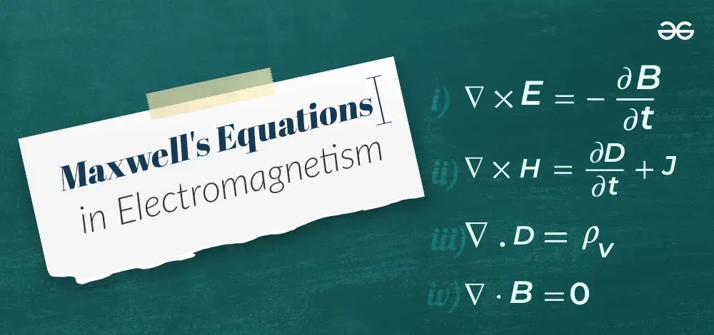
Maxwell’s Equations in Electromagnetism

Maxwell’s Equations are a set of four equations proposed by mathematician and physicist James Clerk Maxwell in 1861 to demonstrate that the electric and magnetic fields are co-dependent and two distinct parts of the same phenomenon known as electromagnetism.

These formulas show how variations in the quantity or velocity of charges can impact magnetic and electric fields. Maxwell went on to establish that light is an electromagnetic wave caused by oscillations in the electric and magnetic fields. Maxwell’s equations give a mathematical model for the operation of all electronic and electromagnetic devices, ranging from power generation to wireless communication.

What are Maxwell’s Equations of Electromagnetism?

Maxwell has combined the four equations that were discovered by Oersted, Ampere, Coulomb, and Faraday. These equations have two forms — one is the partial differential form and the other is the integral form.

These different laws of physics used by Maxwell are,

• Gauss’ law for electrostatics
• Gauss’ law for magnetism
• Faraday’s law of induction
• Ampère’s circuital law

Although not fundamentally discovered by Maxwell, he was the first to combine these to unify two apparently separate physical phenomena. He also applied some corrections to Ampère’s circuital law. Further, he was able to provide a concrete answer to the centuries long debate over the nature of light. Although he unified electricity and magnetism successfully, Maxwell did them in the form of 20 equations. It was Oliver Heaviside, who in 1884, used vector calculus to bring these down to the familiar 4 equation form.

Who was James Clerk Maxwell?

James Clerk Maxwell was one of the most important physicists of the nineteenth century. His creation of the electromagnetic theory and his discovery of the link between light and electromagnetic waves are his most well-known contributions.

Integral form of the Maxwell’s Equations

Lets have a look at the integral form of the Maxwell’s Equations

Gauss’ law for Electrostatics

Gauss’ law for Electrostatics states that the total electric flux through a closed surface is proportional to the enclosed electric charge. Mathematically, this can be expressed as

∇. E = ρ / ε₀

Where E is the electric field, ds is the infinitesimal area element and the closed integral of E over ds gives the electric flux.

Gauss’ law for Magnetism

This law states that the total magnetic flux through a closed surface is zero. This basically means that magnetic monopoles cannot exist. We know that when a magnet is broken down into smaller pieces, each piece will have its own north and south pole – one cannot isolate a single pole. Magnetic poles always exist in pairs and there is no net magnetic field outflow through a closed surface. Mathematically this can be written as

∇. B = 0

Where B is the magnetic field, ds is the infinitesimal area element and the closed integral of B over ds gives the magnetic flux.

Faraday’s law of Induction

Faraday’s law states that changing magnetic flux always generates an EMF that is equal to the negative of the rate of change of the magnetic flux enclosed by the path. The emf is basically the voltage that can be obtained from integrating the electric field. The mathematical form of the Maxwell-Faraday law becomes

∇ × E = − ∂B/ ∂t

This law of electromagnetic induction is the source of all power – the operating principle of electric generators.

Ampere’s Circuital Law

Ampère’s circuital law relates the magnetic field around a closed loop to the electric current passing through the loop. Although named after Ampère, it was actually derived by Maxwell using hydrodynamics(study of liquid flow) in 1861.

∇ × B = μ₀J + μ₀ε₀ ∂E/ ∂t

Where B is the magnetic field, dl is the infinitesimal line element and the line integral of B gives the current flowing through the wire.

Maxwell added a term to this equation known as the displacement current that was defined by the rate of change in electric field. Its origin is not due to actual charge flow, but due to changing electric field. Defined mathematically as,

I_D = ε₀ A . ∂E/∂t

Where I_D is the displacement current, E is the electric field, and A is the surface area.

A prominent example where this comes to play is the case of capacitors. There is no charge transfer between the plates of a capacitor when it first begins to charge. The modified Ampère-Maxwell circuital law now becomes

∮[Tex]\bold{\overrightarrow{\rm B}}[/Tex] . dl = μ₀(I + I_D)

Maxwell’s First Equation – Derived from Gauss’ law of Electrostatics

Gauss’s law for electricity states that the total electric flux out of a closed surface is equal to the charge enclosed divided by the permittivity. Here, the electric flux in an area can be defined as the electric field multiplied by the area of the surface projected in a plane and perpendicular to the field.

As per the Gauss’s Law of Electrostatics

∯ [Tex]\overrightarrow{\rm E} [/Tex].ds = Q/ε₀ —-(1)

Applying divergence theorem,

∯ [Tex]\overrightarrow{\rm E} [/Tex]. ds = ∭ ∇. [Tex]\overrightarrow{\rm E} [/Tex] dv —-(2)

From equations (1) and (2) we get,

∭ ∇. [Tex]\overrightarrow{\rm E} [/Tex] dv = Q /ε₀ dv

we need to define charge as the integral of volume charge density Q = ∭_v ρ dV

∇. [Tex]\overrightarrow{\rm E} [/Tex] = ρ /ε₀ (Maxwell’s First Equation)

Maxwell’s Second Equation – Derived from Gauss’ law of Magnetism

According to Gauss’ law of Magnetism, magnetic field flux through any closed surface is zero which is equivalent to the statement that magnetic field lines are continuous. They have no beginning or end. Thus any magnetic field line entering the region enclosed by the surface must leave it too.

From Gauss’s Law of Magnetism

∯ [Tex]\overrightarrow{\rm B} [/Tex]. ds = 0 —-(1)

Applying divergence theorem,

∯ [Tex]\overrightarrow{\rm B} [/Tex]. ds = ∭ ∇. [Tex]\overrightarrow{\rm B} [/Tex] dv —-(2)

From equations (1) and (2) we get,

∭ ∇. [Tex]\overrightarrow{\rm B} [/Tex] dv = 0

Here to satisfy the above equation we can either have

∭ dv= 0 or ∇. [Tex]\overrightarrow{\rm B} [/Tex] = 0

Since the volume of any body or object can never be zero. We get our Second Maxwell Equation,

∇. [Tex]\overrightarrow{\rm B} [/Tex] = 0 (Maxwell’s Second Equation)

Maxwell’s Third Equation – Derived from Faraday’s law of Induction

According to Faraday’s Law of Induction , a change in magnetic field induces an electromotive force which is called emf in short. This generates an electric field.

The direction of the EMF tries to oppose the change. The electric field arising from a changing magnetic field represents field lines that form closed loops that do not have any beginning or end.

From Faraday’s law of Induction

∮ [Tex]\overrightarrow{\rm E} [/Tex]. dl = − ∬ d[Tex]\overrightarrow{\rm B} [/Tex]/ dt. ds —-(1)

Applying Stokes Theorem,

∮ [Tex]\overrightarrow{\rm E} [/Tex] .dl = ∬ (∇ × [Tex]\overrightarrow{\rm E} [/Tex]) .ds —-(2)

From equations (1) and (2) we get,

∬ ( ▽× [Tex]\overrightarrow{\rm E} [/Tex]) ds = ∬ – [Tex]\overrightarrow{\rm B} [/Tex]/dt .ds

▽× [Tex]\overrightarrow{\rm E} [/Tex] = – [Tex]\overrightarrow{\rm B} [/Tex]/dt (Maxwell’s Third Equation)

Maxwell’s Fourth Equation – Derived from Ampere’s Circuital Law

According to Ampere Circuital law, moving charges or changing electric fields generate magnetic fields. This equation considers Ampère’s law.

From Ampere Circuital Law,

∮ [Tex]\overrightarrow{\rm B} [/Tex]. dl = μ₀(I + I_D) —-(1)

where i = ∮_s J . ds

Applying Stokes Theorem,

∮ [Tex]\overrightarrow{\rm B} [/Tex] .dl = ∮s ( ∇ × [Tex]\overrightarrow{\rm B} [/Tex] ) .ds —-(2)

From equation 1 and 2 we get ,

∮_s ( ∇ × [Tex]\overrightarrow{\rm B} [/Tex] ).ds = μ₀ (I + I_D)

∮_s ( ∇ × [Tex]\overrightarrow{\rm B} [/Tex] ).ds = μ₀ ( J + J_D)

∮_s [( ∇ × [Tex]\overrightarrow{\rm B} [/Tex] ) – μ₀ ( J + J_D) ].ds =0

∇ × [Tex]\overrightarrow{\rm B} [/Tex] = μ₀ ( J + J_D) —-(3)

where JD is the displacement current density and it value is J_D= ϵ₀ (∂[Tex]\overrightarrow{\rm E} [/Tex]/∂t) ,putting this value in equation (3) we get,

∇ × [Tex]\overrightarrow{\rm B} [/Tex] = μ₀ J + μ₀ ϵ₀ (∂[Tex]\overrightarrow{\rm E} [/Tex]/∂t) (Maxwell’s Fourth Equation)

Maxwell’s Equations: Differential and Integral Form

The Differential and Integral Form of Maxwell Equation are stated below:

Name of law	Differential Form	Integral Form
Gauss’ law for Electricity	∇. E = ρ / ε0	∮ E. ds = Q/ε0
Gauss’ law for Magnetism	∇. B = 0	∮ B. ds = 0
Faraday’s law	∇ x E = − ∂B/ ∂t	∮ E. dl = − ∫ ∂B/∂t . ds
Ampere’s law	∇ x B = μ0J + μ0ε0 ∂E/ ∂t	∮ B. dl = μ (I + ID)

Applications of Maxwell Equations

The applications of Maxwell Equations are as follows

• Electric motors, wireless communication, lenses, radar, and other electric, optical, and radio technologies are all represented mathematically by the equations.
• They explain how electric and magnetic fields are created by charges, currents, and changes in the field.
• A changing magnetic field always generates an electric field, and a changing electric field always induces a magnetic field, according to Maxwell’s equations.

Merits of Maxwell’s Equations

Merits of Maxwell’s Equations are as follows:

• The relationship between the theories of electricity and magnetism is demonstrated by Maxwell’s equations.
• Maxwell’s equations were used to predict and explain a wide range of electromagnetic phenomena, such as the behaviour of electric circuits and the propagation of electromagnetic waves, which include light.
• Classical electrodynamics is based on these equations. They are required in order to understand how charges and currents generate electromagnetic fields.
• Maxwell’s equations, which predicted electromagnetic waves, made it feasible for light to emerge as an electromagnetic wave and paved the path for the development of technologies like radio, television, and wireless communication.
• Maxwell’s equations, which are essential to modern physics, have inspired the creation of several theories, including as special relativity and quantum mechanics.

Limitations of Maxwell’s Equations

The limitations of Maxwell’s Equations are as follows:

• Even though Maxwell’s equations are derived from classical electrodynamics, extending them to extremely small scales (quantum electrodynamics) and extremely high speeds (relativistic electrodynamics) requires the use of more complex theories.
• Quantum effects are not taken into consideration by Maxwell’s equations.
• Maxwell’s equations are based on a number of assumptions and simplifications, including the idealized properties of materials and the absence of magnetic monopoles. It’s possible that these assumptions don’t always accurately depict events that take place in reality.
• Although Maxwell’s equations are straightforward, it can be difficult to solve them for complex geometries and boundary conditions.
• Maxwell’s equations form a classical theory and do not incorporate concepts from gravitational force quantum mechanics.

Conclusion: Maxwell’s Equations in Electromagnetism

To understand these Maxwell’s equations, first we need to completely understand the underlying laws that were discovered by Coulomb, Oersted, Ampere, and Faraday. These are very basic and easy-to-understand laws of physics and are used in everyday activities like in the smallest motors, capacitors, and many other activities.

Read More,

• Ampere’s Law
• Gauss Law
• Applications of Gauss Law

Maxwell’s Equations Solved Examples

Let’s solve some example problems on Maxwell’s Equations:

Example 1: In an electromagnetic wave, the electric field of amplitude 5.4 V/m oscillates with a frequency of 3.0 x 10¹⁰ Hz. Calculate the energy density of the wave.

Solution:

The amplitude of the electric field, E₀ = 5.4 V/m

Frequency of the electric field, f = 3.0 × 10¹⁰ Hz

According to Maxwell’s equations, energy density is given by

Energy density = ∈₀E₀²

Where

∈₀ is the absolute permittivity of the free space = 8.854 × 10^-12 C²N/m²

E₀ is the amplitude of the electric field

On substituting the values, we get

Energy density = (8.854 x 10^-12 ) × (5.4)²

Energy density = 2.58 × 10^-10 J/m³

Example 2: If the velocity of a charged particle in perpendicular electric and magnetic field is 7.5 X 10⁶m/s and the Electric field is 4 X 10⁶ N/c, what should be the value of magnetic field for velocity sector?

Solution:

As we know, for velocity selector, v = E / B

Therefore, B = E/v

⇒ B = 4 × 10⁶ /7.5 × 10⁶

⇒ B = 0.53 T

Example 3: A point charge of 10^-6 C is at the centre of a cubical Gaussian surface of sides 0.5 m. What is the flux for the surface?

Solution:

We know that for a Gaussian surface, flux = q/ε

Here, q = 10^-6 C and ε = 8.85 × 10^-12 C/Nm²

Therefore, flux = 10^-6/8.85 × 10^-12

= 1.12 × 10⁵ Nm²/C.

Maxwell’s Equations Practice Questions

Q1: If the velocity of a charged particle in a perpendicular electric and magnetic field is 7.5 x 10⁶ m/s and the Electric field is 5 x 10⁶ N/C, what should be the value of the magnetic field for the velocity sector?

Q2: In an electromagnetic wave, the electric field of amplitude 5 V/m oscillates with a frequency of 2.5 x 10¹⁰ Hz. Calculate the energy density of the wave.

FAQs on Maxwell’s Equations in Electromagnetism

What are the Maxwell’s Electromagnetic Equations?

Maxwell’s electromagnetic equations describe the behavior of electric and magnetic fields. They include Gauss’s law, Gauss’s law for magnetism, Faraday’s law of electromagnetic induction, and Ampère’s law with Maxwell’s addition.

How many Maxwell’s Equation are There?

Maxwell’s equations consist of four fundamental equations: Gauss’s law for electricity, Gauss’s law for magnetism, Faraday’s law of electromagnetic induction, and Ampère’s law.

What are the Four Maxwell’s Equations?

The four Maxwell’s Equations are:

1. ∇. E = ρ / ε₀
2. ∇. B = 0
3. ∇ x E = − ∂B/ ∂t
4. ∇ x B = μ₀J + μ₀ε₀ ∂E/ ∂t

What is Meant by Scalar Magnetic Flux?

Scalar Magnetic Flux are the circular magnetic fields produced by current -carrying conductors.

What is Displacement Current?

Displacement current is defined by the rate of change in electric field and is a source of magnetic field, like conventional current. Defined mathematically as,

I_D= ε₀A ∂E/∂t