Attacks fall into four main categories:
- #DOS: denial-of-service, e.g. syn flood;
- #R2L: unauthorized access from a remote machine, e.g. guessing password;
- #U2R: unauthorized access to local superuser (root) privileges, e.g., various “buffer overflow” attacks;
- #probing: surveillance and another probing, e.g., port scanning.
Dataset Used : KDD Cup 1999 dataset
Dataset Description: Data files:
- kddcup.names : A list of features.
- kddcup.data.gz : The full data set
- kddcup.data_10_percent.gz : A 10% subset.
- kddcup.newtestdata_10_percent_unlabeled.gz
- kddcup.testdata.unlabeled.gz
- kddcup.testdata.unlabeled_10_percent.gz
- corrected.gz : Test data with corrected labels.
- training_attack_types : A list of intrusion types.
- typo-correction.txt : A brief note on a typo in the data set that has been corrected
Features:
| feature name |
description |
type |
| duration |
length (number of seconds) of the connection |
continuous |
| protocol_type |
type of the protocol, e.g. tcp, udp, etc. |
discrete |
| service |
network service on the destination, e.g., http, telnet, etc. |
discrete |
| src_bytes |
number of data bytes from source to destination |
continuous |
| dst_bytes |
number of data bytes from destination to source |
continuous |
| flag |
normal or error status of the connection |
discrete |
| land |
1 if connection is from/to the same host/port; 0 otherwise |
discrete |
| wrong_fragment |
number of “wrong” fragments |
continuous |
| urgent |
number of urgent packets |
continuous |
Table 1: Basic features of individual TCP connections.
| feature name |
description |
type |
| hot |
number of “hot” indicators |
continuous |
| num_failed_logins |
number of failed login attempts |
continuous |
| logged_in |
1 if successfully logged in; 0 otherwise |
discrete |
| num_compromised |
number of “compromised” conditions |
continuous |
| root_shell |
1 if root shell is obtained; 0 otherwise |
discrete |
| su_attempted |
1 if “su root” command attempted; 0 otherwise |
discrete |
| num_root |
number of “root” accesses |
continuous |
| num_file_creations |
number of file creation operations |
continuous |
| num_shells |
number of shell prompts |
continuous |
| num_access_files |
number of operations on access control files |
continuous |
| num_outbound_cmds |
number of outbound commands in an ftp session |
continuous |
| is_hot_login |
1 if the login belongs to the “hot” list; 0 otherwise |
discrete |
| is_guest_login |
1 if the login is a “guest”login; 0 otherwise |
discrete |
Table 2: Content features within a connection suggested by domain knowledge.
| feature name |
description |
type |
| count |
number of connections to the same host as the current connection in the past two seconds |
continuous |
| |
Note: The following features refer to these same-host connections. |
|
| serror_rate |
% of connections that have “SYN” errors |
continuous |
| rerror_rate |
% of connections that have “REJ” errors |
continuous |
| same_srv_rate |
% of connections to the same service |
continuous |
| diff_srv_rate |
% of connections to different services |
continuous |
| srv_count |
number of connections to the same service as the current connection in the past two seconds |
continuous |
| |
Note: The following features refer to these same-service connections. |
|
| srv_serror_rate |
% of connections that have “SYN” errors |
continuous |
| srv_rerror_rate |
% of connections that have “REJ” errors |
continuous |
| srv_diff_host_rate |
% of connections to different hosts |
continuous |
Table 3: Traffic features computed using a two-second time window.
Various Algorithms Applied: Gaussian Naive Bayes, Decision Tree, Random Forest, Support Vector Machine, Logistic Regression.
Approach Used: I have applied various classification algorithms that are mentioned above on the KDD dataset and compare there results to build a predictive model.
Step 1 – Data Preprocessing:
Code: Importing libraries and reading features list from ‘kddcup.names’ file.
import os
import pandas as pd
import numpy as np
import matplotlib.pyplot as plt
import seaborn as sns
import time
with open("..\\kddcup.names", 'r') as f:
print(f.read())
|
Code: Appending columns to the dataset and adding a new column name ‘target’ to the dataset.
cols =
columns =[]
for c in cols.split(', '):
if(c.strip()):
columns.append(c.strip())
columns.append('target')
print(len(columns))
|
Output:
42
Code: Reading the ‘attack_types’ file.
with open("..\\training_attack_types", 'r') as f:
print(f.read())
|
Output:
back dos
buffer_overflow u2r
ftp_write r2l
guess_passwd r2l
imap r2l
ipsweep probe
land dos
loadmodule u2r
multihop r2l
neptune dos
nmap probe
perl u2r
phf r2l
pod dos
portsweep probe
rootkit u2r
satan probe
smurf dos
spy r2l
teardrop dos
warezclient r2l
warezmaster r2l
Code: Creating a dictionary of attack_types
attacks_types = {
'normal': 'normal',
'back': 'dos',
'buffer_overflow': 'u2r',
'ftp_write': 'r2l',
'guess_passwd': 'r2l',
'imap': 'r2l',
'ipsweep': 'probe',
'land': 'dos',
'loadmodule': 'u2r',
'multihop': 'r2l',
'neptune': 'dos',
'nmap': 'probe',
'perl': 'u2r',
'phf': 'r2l',
'pod': 'dos',
'portsweep': 'probe',
'rootkit': 'u2r',
'satan': 'probe',
'smurf': 'dos',
'spy': 'r2l',
'teardrop': 'dos',
'warezclient': 'r2l',
'warezmaster': 'r2l',
}
|
Code: Reading the dataset(‘kddcup.data_10_percent.gz’) and adding Attack Type feature in the training dataset where attack type feature has 5 distinct values i.e. dos, normal, probe, r2l, u2r.
path = "..\\kddcup.data_10_percent.gz"
df = pd.read_csv(path, names = columns)
df['Attack Type'] = df.target.apply(lambda r:attacks_types[r[:-1]])
df.head()
|
Code: Shape of dataframe and getting data type of each feature
Output:
(494021, 43)
Code: Finding missing values of all features.
Output:
duration                       0
protocol_type                  0
service                        0
flag                           0
src_bytes                      0
dst_bytes                      0
land                           0
wrong_fragment                 0
urgent                         0
hot                            0
num_failed_logins              0
logged_in                      0
num_compromised                0
root_shell                     0
su_attempted                   0
num_root                       0
num_file_creations             0
num_shells                     0
num_access_files               0
num_outbound_cmds              0
is_host_login                  0
is_guest_login                 0
count                          0
srv_count                      0
serror_rate                    0
srv_serror_rate                0
rerror_rate                    0
srv_rerror_rate                0
same_srv_rate                  0
diff_srv_rate                  0
srv_diff_host_rate             0
dst_host_count                 0
dst_host_srv_count             0
dst_host_same_srv_rate         0
dst_host_diff_srv_rate         0
dst_host_same_src_port_rate    0
dst_host_srv_diff_host_rate    0
dst_host_serror_rate           0
dst_host_srv_serror_rate       0
dst_host_rerror_rate           0
dst_host_srv_rerror_rate       0
target                         0
Attack Type                    0
dtype: int64
No missing value found, so we can further proceed to our next step.
Code: Finding Categorical Features
num_cols = df._get_numeric_data().columns
cate_cols = list(set(df.columns)-set(num_cols))
cate_cols.remove('target')
cate_cols.remove('Attack Type')
cate_cols
|
Output:
['service', 'flag', 'protocol_type']
Visualizing Categorical Features using bar graph
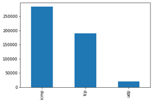
Protocol type: We notice that ICMP is the most present in the used data, then TCP and almost 20000 packets of UDP type
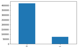
logged_in (1 if successfully logged in; 0 otherwise): We notice that just 70000 packets are successfully logged in.
Target Feature Distribution:
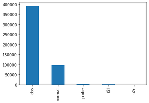
Attack Type(The attack types grouped by attack, it’s what we will predict)
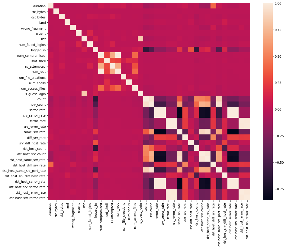
Code: Data Correlation – Find the highly correlated variables using heatmap and ignore them for analysis.
df = df.dropna('columns')
df = df[[col for col in df if df[col].nunique() > 1]]
corr = df.corr()
plt.figure(figsize =(15, 12))
sns.heatmap(corr)
plt.show()
|
Output:
Code:
df.drop('num_root', axis = 1, inplace = True)
df.drop('srv_serror_rate', axis = 1, inplace = True)
df.drop('srv_rerror_rate', axis = 1, inplace = True)
df.drop('dst_host_srv_serror_rate', axis = 1, inplace = True)
df.drop('dst_host_serror_rate', axis = 1, inplace = True)
df.drop('dst_host_rerror_rate', axis = 1, inplace = True)
df.drop('dst_host_srv_rerror_rate', axis = 1, inplace = True)
df.drop('dst_host_same_srv_rate', axis = 1, inplace = True)
|
Output:
Code: Feature Mapping – Apply feature mapping on features such as : ‘protocol_type’ & ‘flag’.
pmap = {'icmp':0, 'tcp':1, 'udp':2}
df['protocol_type'] = df['protocol_type'].map(pmap)
|
Code:
fmap = {'SF':0, 'S0':1, 'REJ':2, 'RSTR':3, 'RSTO':4, 'SH':5, 'S1':6, 'S2':7, 'RSTOS0':8, 'S3':9, 'OTH':10}
df['flag'] = df['flag'].map(fmap)
|
Output:
Code: Remove irrelevant features such as ‘service’ before modelling
df.drop('service', axis = 1, inplace = True)
|
Step 2 – Modelling
Code: Importing libraries and splitting the dataset
from sklearn.model_selection import train_test_split
from sklearn.preprocessing import MinMaxScaler
|
Code:
df = df.drop(['target', ], axis = 1)
print(df.shape)
y = df[['Attack Type']]
X = df.drop(['Attack Type', ], axis = 1)
sc = MinMaxScaler()
X = sc.fit_transform(X)
X_train, X_test, y_train, y_test = train_test_split(X, y, test_size = 0.33, random_state = 42)
print(X_train.shape, X_test.shape)
print(y_train.shape, y_test.shape)
|
Output:
(494021, 31)
(330994, 30) (163027, 30)
(330994, 1) (163027, 1)
Apply various machine learning classification algorithms such as Support Vector Machines, Random Forest, Naive Bayes, Decision Tree, Logistic Regression to create different models.
Code: Python implementation of Gaussian Naive Bayes
from sklearn.naive_bayes import GaussianNB
from sklearn.metrics import accuracy_score
clfg = GaussianNB()
start_time = time.time()
clfg.fit(X_train, y_train.values.ravel())
end_time = time.time()
print("Training time: ", end_time-start_time)
|
Output:
Training time: 1.1145250797271729
Code:
start_time = time.time()
y_test_pred = clfg.predict(X_train)
end_time = time.time()
print("Testing time: ", end_time-start_time)
|
Output:
Testing time: 1.543299674987793
Code:
print("Train score is:", clfg.score(X_train, y_train))
print("Test score is:", clfg.score(X_test, y_test))
|
Output:
Train score is: 0.8795114110829804
Test score is: 0.8790384414851528
Code: Python implementation of Decision Tree
from sklearn.tree import DecisionTreeClassifier
clfd = DecisionTreeClassifier(criterion ="entropy", max_depth = 4)
start_time = time.time()
clfd.fit(X_train, y_train.values.ravel())
end_time = time.time()
print("Training time: ", end_time-start_time)
|
Output:
Training time: 2.4408750534057617
start_time = time.time()
y_test_pred = clfd.predict(X_train)
end_time = time.time()
print("Testing time: ", end_time-start_time)
|
Output:
Testing time: 0.1487727165222168
print("Train score is:", clfd.score(X_train, y_train))
print("Test score is:", clfd.score(X_test, y_test))
|
Output:
Train score is: 0.9905829108684749
Test score is: 0.9905230421954646
Code: Python code implementation of Random Forest
from sklearn.ensemble import RandomForestClassifier
clfr = RandomForestClassifier(n_estimators = 30)
start_time = time.time()
clfr.fit(X_train, y_train.values.ravel())
end_time = time.time()
print("Training time: ", end_time-start_time)
|
Output:
Training time: 17.084914684295654
start_time = time.time()
y_test_pred = clfr.predict(X_train)
end_time = time.time()
print("Testing time: ", end_time-start_time)
|
Output:
Testing time: 0.1487727165222168
print("Train score is:", clfr.score(X_train, y_train))
print("Test score is:", clfr.score(X_test, y_test))
|
Output:
Train score is: 0.99997583037759
Test score is: 0.9996933023364228
Code: Python implementation of Support Vector Classifier
from sklearn.svm import SVC
clfs = SVC(gamma = 'scale')
start_time = time.time()
clfs.fit(X_train, y_train.values.ravel())
end_time = time.time()
print("Training time: ", end_time-start_time)
|
Output:
Training time: 218.26840996742249
Code:
start_time = time.time()
y_test_pred = clfs.predict(X_train)
end_time = time.time()
print("Testing time: ", end_time-start_time)
|
Output:
Testing time: 126.5087513923645
Code:
print("Train score is:", clfs.score(X_train, y_train))
print("Test score is:", clfs.score(X_test, y_test))
|
Output:
Train score is: 0.9987552644458811
Test score is: 0.9987916112055059
Code: Python implementation of Logistic Regression
from sklearn.linear_model import LogisticRegression
clfl = LogisticRegression(max_iter = 1200000)
start_time = time.time()
clfl.fit(X_train, y_train.values.ravel())
end_time = time.time()
print("Training time: ", end_time-start_time)
|
Output:
Training time: 92.94222283363342
Code:
start_time = time.time()
y_test_pred = clfl.predict(X_train)
end_time = time.time()
print("Testing time: ", end_time-start_time)
|
Output:
Testing time: 0.09605908393859863
Code:
print("Train score is:", clfl.score(X_train, y_train))
print("Test score is:", clfl.score(X_test, y_test))
|
Output:
Train score is: 0.9935285835997028
Test score is: 0.9935286792985211
Code: Python implementation of Gradient Descent
from sklearn.ensemble import GradientBoostingClassifier
clfg = GradientBoostingClassifier(random_state = 0)
start_time = time.time()
clfg.fit(X_train, y_train.values.ravel())
end_time = time.time()
print("Training time: ", end_time-start_time)
|
Output:
Training time: 633.2290260791779
start_time = time.time()
y_test_pred = clfg.predict(X_train)
end_time = time.time()
print("Testing time: ", end_time-start_time)
|
Output:
Testing time: 2.9503915309906006
print("Train score is:", clfg.score(X_train, y_train))
print("Test score is:", clfg.score(X_test, y_test))
|
Output:
Train score is: 0.9979304760811374
Test score is: 0.9977181693829856
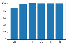
Code: Analyse the training and testing accuracy of each model.
names = ['NB', 'DT', 'RF', 'SVM', 'LR', 'GB']
values = [87.951, 99.058, 99.997, 99.875, 99.352, 99.793]
f = plt.figure(figsize =(15, 3), num = 10)
plt.subplot(131)
plt.bar(names, values)
|
Output:

Code:
names = ['NB', 'DT', 'RF', 'SVM', 'LR', 'GB']
values = [87.903, 99.052, 99.969, 99.879, 99.352, 99.771]
f = plt.figure(figsize =(15, 3), num = 10)
plt.subplot(131)
plt.bar(names, values)
|
Output:
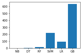
Code: Analyse the training and testing time of each model.
names = ['NB', 'DT', 'RF', 'SVM', 'LR', 'GB']
values = [1.11452, 2.44087, 17.08491, 218.26840, 92.94222, 633.229]
f = plt.figure(figsize =(15, 3), num = 10)
plt.subplot(131)
plt.bar(names, values)
|
Output:
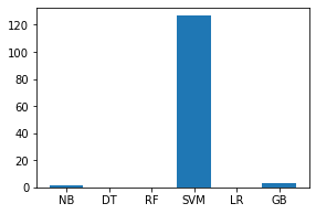
Code:
names = ['NB', 'DT', 'RF', 'SVM', 'LR', 'GB']
values = [1.54329, 0.14877, 0.199471, 126.50875, 0.09605, 2.95039]
f = plt.figure(figsize =(15, 3), num = 10)
plt.subplot(131)
plt.bar(names, values)
|
Output:
Implementation Link: https://github.com/mudgalabhay/intrusion-detection-system/blob/master/main.ipynb
Conclusion: The above analysis of different models states that the Decision Tree model best fits our data considering both accuracy and time complexity.
Links: The complete code is uploaded on my github account – https://github.com/mudgalabhay/intrusion-detection-system
Share your thoughts in the comments
Please Login to comment...