Alzheimer’s detection Using Machine Learning

Alzheimer’s disease is a neurodegenerative disorder characterized by progressive cognitive decline and memory loss. Detecting Alzheimer’s disease early is crucial for timely intervention and treatment. While I can provide some general information on Alzheimer’s detection, it’s important to consult medical professionals for accurate diagnosis and advice.

Alzheimer’s detection

Machine learning has shown promise in aiding the detection of Alzheimer’s disease. In this article, we will apply RandomForestClassifier and LocalOutlierFactor to detect Alzheimer’s disease.

Steps:

• Launch the Jupyter Notebook or Colab
• Download the dataset from the given link.
• Import required libraries.
• Preprocess the dataset.
• Perform Outlier detection.
• Train and Test model.
• Evaluate the model.
• You can use visualization techniques (option – if needed)

Download the dataset from here: Dataset

COL	FULL-FORMS
Group	Nondemented or Demented
EDUC	Years of education
SES	Socioeconomic Status
MMSE	Mini-Mental State Examination
CDR	Clinical Dementia Rating
eTIV	Estimated Total Intracranial Volume
nWBV	Normalize Whole Brain Volume
ASF	Atlas Scaling Factor

The dataset contains 373 rows with 14 fields which contain Group fields with classes Demented and Non-Demented where we need to work on them.

Import required libraries:

Python3

#import required packages

import pandas as pd
import numpy as np
from sklearn.model_selection import train_test_split
from sklearn.preprocessing import MinMaxScaler, OneHotEncoder
from sklearn.compose import ColumnTransformer
from sklearn.pipeline import Pipeline
from sklearn.ensemble import RandomForestClassifier
from sklearn.neighbors import LocalOutlierFactor
from sklearn.metrics import accuracy_score, precision_score, recall_score, f1_score, confusion_matrix
import seaborn as sns
import matplotlib.pyplot as plt

We have imported the required packages.

Load the dataset

Python3

# Loading into a dataframe
df = pd.read_csv('oasis_longitudinal.csv')

# Have a peek at the data
# Returns fist 5 columns
print(df.head())

Output:

  Subject ID         MRI ID        Group  Visit  MR Delay M/F Hand  Age  EDUC  \
0  OAS2_0001  OAS2_0001_MR1  Nondemented      1         0   M    R   87    14   
1  OAS2_0001  OAS2_0001_MR2  Nondemented      2       457   M    R   88    14   
2  OAS2_0002  OAS2_0002_MR1     Demented      1         0   M    R   75    12   
3  OAS2_0002  OAS2_0002_MR2     Demented      2       560   M    R   76    12   
4  OAS2_0002  OAS2_0002_MR3     Demented      3      1895   M    R   80    12   
   SES  MMSE  CDR  eTIV   nWBV    ASF  
0  2.0  27.0  0.0  1987  0.696  0.883  
1  2.0  30.0  0.0  2004  0.681  0.876  
2  NaN  23.0  0.5  1678  0.736  1.046  
3  NaN  28.0  0.5  1738  0.713  1.010  
4  NaN  22.0  0.5  1698  0.701  1.034  

Check the data info

Python3

df.info()

Output:

<class 'pandas.core.frame.DataFrame'>
RangeIndex: 373 entries, 0 to 372
Data columns (total 15 columns):
 #   Column      Non-Null Count  Dtype  
---  ------      --------------  -----  
 0   Subject ID  373 non-null    object 
 1   MRI ID      373 non-null    object 
 2   Group       373 non-null    object 
 3   Visit       373 non-null    int64  
 4   MR Delay    373 non-null    int64  
 5   M/F         373 non-null    object 
 6   Hand        373 non-null    object 
 7   Age         373 non-null    int64  
 8   EDUC        373 non-null    int64  
 9   SES         354 non-null    float64
 10  MMSE        371 non-null    float64
 11  CDR         373 non-null    float64
 12  eTIV        373 non-null    int64  
 13  nWBV        373 non-null    float64
 14  ASF         373 non-null    float64
dtypes: float64(5), int64(5), object(5)
memory usage: 43.8+ KB

Preprocessing the dataset

Dropping irrelevant columns

Python3

# Dropping the list of columns mentioned
df = df.drop(['Subject ID', 'MRI ID', 'Hand', 'Visit', 'MR Delay'], axis=1)
df.shape

Output:

(373, 10)

Check Group Features

Python3

df['Group'].value_counts()

Output:

Group
Nondemented    190
Demented       146
Converted       37
Name: count, dtype: int64

Replace the “Converted” with “Demented”

Python3

df['Group'] = df['Group'].replace(['Converted'], ['Demented'])

Replace Categorical String Data with Numerical Data

• df[‘M/F’] = df[‘M/F’].replace([‘F’, ‘M’], [0, 1]): Replaces the values in the ‘M/F’ (Male/Female) column, ‘F’ with 0 and ‘M’ with 1. This helps to convert categorical values into binary format.
• df[‘Group’] = df[‘Group’].replace([‘Demented’, ‘Nondemented’], [1, 0]): Replaces the values ‘Demented’ with 1 and ‘Nondemented’ with 0 in the ‘Group’ column for binary classification.

Python3

df['M/F'] = df['M/F'].replace(['F', 'M'], [0, 1])
df['Group'] = df['Group'].replace(['Demented', 'Nondemented'], [1, 0])

Check for Null Values

Python3

df.isnull().sum()

Output:

Group     0
M/F       0
Age       0
EDUC      0
SES      19
MMSE      2
CDR       0
eTIV      0
nWBV      0
ASF       0
dtype: int64

Imputating the missing values

As we can see that only the SES column has null values. Because SES denotes ranks of Socioeconomic Status, It is a categorical feature. So, We can replace the null values of SES with its mode.

Fill the MMSE null values with its Median

Python3

# Fill with mode values
df['SES'] = df['SES'].fillna(value= df['SES'].mode().iloc[0])
# Fill with mean values
df['MMSE'] = df['MMSE'].fillna(value =df['MMSE'].median())

Separate Input Features and Target Variables Group

Python3

Y = df['Group'].values
X = df[['M/F', 'Age', 'EDUC', 'SES', 'MMSE', 'eTIV', 'nWBV', 'ASF']]

Y represents the target variable – labels as a Numpy array and X represents the list of selected columns as a matrix which is used for the classification task.

Numerical and Categorical Features

Python3

numerical_features = ['Age', 'EDUC',  'MMSE', 'eTIV', 'nWBV', 'ASF']
categorical_features = ['M/F', 'SES']

Treating Outliers

outlier_detector = LocalOutlierFactor(contamination=0.05): Creating an instance of the Local Outlier Factor (LOF) algorithm for outlier detection. The contamination parameter is set to 0.05, which means we are expecting 5% outliers.

outliers = outlier_detector.fit_predict(X): This step calculates the outlier scores for each sample. This also gives and assigns a label of -1 for outliers and 1 for inliers.

Python3

outlier_detector = LocalOutlierFactor(contamination=0.05)
outliers = outlier_detector.fit_predict(X)
X = X[outliers == 1]
Y = Y[outliers == 1]

Standardize and One Hot Encoding

The next two steps represent that we are selecting only inliers for further processing. This step of code creates transformers for categorical numerical and numerical features and helps in training the model consistently.

• MinMaxScalar helps to scale numerical features.
• OneHotEncoder is used to encode categorical features.
• These transformers are merged using a ColumnTransformer.

Python3

#numerical transformer and categorical transformer
numerical = MinMaxScaler()
categorical = OneHotEncoder(drop='first')

p = ColumnTransformer(transformers=[('num', numerical, numerical_features),
                                    ('cat', categorical, categorical_features)])

Visualizing dataset target class details:

Python3

sns.countplot(data=df, x='Group')
plt.title("Distribution of Classes")
plt.xlabel("Group")
plt.ylabel("Count")
plt.show()

Output:

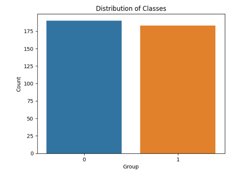
Target class distribution

Splitting data for training and testing:

Python3

X_train, X_test, Y_train, Y_test = train_test_split(X, Y, random_state=0)

By default, 75% for training and 25% for testing.

Build the Pipeline

Building a pipeline for usage with Random Forest classifier and Preprocessor, then fit the model.

Python3

pl_rf = Pipeline(steps=[('preprocessor', p),('classifier', RandomForestClassifier(random_state=0))])

pl_rf.fit(X_train, Y_train)

Predictions:

Python3

Y_pred_rf = pl_rf.predict(X_test)

Evaluating the model:

Python3

print("Accuracy:", accuracy_score(Y_test, Y_pred_rf))
print("Precision:", precision_score(Y_test, Y_pred_rf))
print("Recall:", recall_score(Y_test, Y_pred_rf))
print("F1 Score:", f1_score(Y_test, Y_pred_rf))

Output:

Accuracy: 0.8651685393258427
Precision: 0.825
Recall: 0.868421052631579
F1 Score: 0.8461538461538461

Confusion Matrix:

Python3

cnf = confusion_matrix(Y_test, Y_pred_rf)

sns.heatmap(cnf, annot=True, fmt='d', cmap='Green')
plt.title("Confusion Matrix for above model")
plt.xlabel("Predicted")
plt.ylabel("True")
plt.show()

Output:

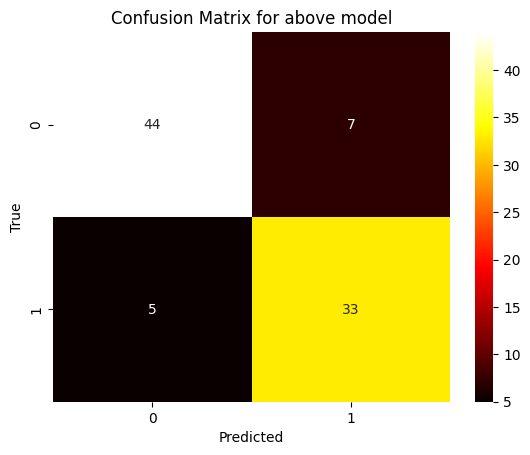
Confusion Matrix