Dog Breed Classification using Transfer Learning

In this article, we will learn how to build a classifier using the Transfer Learning technique which can classify among different breeds of dogs. This project has been developed using collab and the dataset has been taken from Kaggle whose link has been provided as well.

Transfer Learning

In a convolutional neural network, the main task of the convolutional layers is to enhance the important features of an image. If a particular filter is used to identify the straight lines in an image then it will work for other images as well this is particularly what we do in transfer learning. There are models which are developed by researchers by regress hyperparameter tuning and training for weeks on millions of images belonging to 1000 different classes like imagenet dataset. A model that works well for one computer vision task proves to be good for others as well. Because of this reason, we leverage those trained convolutional layers parameters and tuned hyperparameters for our task to obtain higher accuracy.

Importing Libraries

Python libraries make it very easy for us to handle the data and perform typical and complex tasks with a single line of code.

• Pandas – This library helps to load the data frame in a 2D array format and has multiple functions to perform analysis tasks in one go.
• Numpy – Numpy arrays are very fast and can perform large computations in a very short time.
• Matplotlib – This library is used to draw visualizations.
• Sklearn – This module contains multiple libraries having pre-implemented functions to perform tasks from data preprocessing to model development and evaluation.
• OpenCV – This is an open-source library mainly focused on image processing and handling.
• Tensorflow – This is an open-source library that is used for Machine Learning and Artificial intelligence and provides a range of functions to achieve complex functionalities with single lines of code.

Python3

import numpy as np
import pandas as pd
import matplotlib.pyplot as plt
import seaborn as sb

from sklearn.preprocessing import LabelEncoder
from sklearn.model_selection import train_test_split

import cv2
import tensorflow as tf
from tensorflow import keras
from keras import layers
from functools import partial

import warnings
warnings.filterwarnings('ignore')
AUTO = tf.data.experimental.AUTOTUNE

Importing Dataset

The dataset which we will use here has been taken from – https://www.kaggle.com/competitions/dog-breed-identification/data. This dataset includes 10,000 images of 120 different breeds of dogs. In this data set, we have a training images folder. test image folder and a CSV file that contains information regarding the image and the breed it belongs to.

Python3

from zipfile import ZipFile
data_path = 'dog-breed-identification.zip'

with ZipFile(data_path, 'r') as zip:
    zip.extractall()
    print('The data set has been extracted.')

Output:

The data set has been extracted.

Python3

df = pd.read_csv('labels.csv')
df.head()

Output:

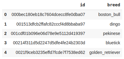
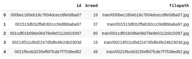
First Five rows of the dataset

Python3

df.shape

Output:

(10222, 2)

Let’s check the number of unique breeds of dog images we have in the training data.

Python3

df['breed'].nunique()

Output:

120

So, here we can see that there are 120 unique breed data which has been provided to us.

Python3

plt.figure(figsize=(10, 5))
df['breed'].value_counts().plot.bar()
plt.axis('off')
plt.show()

Output:

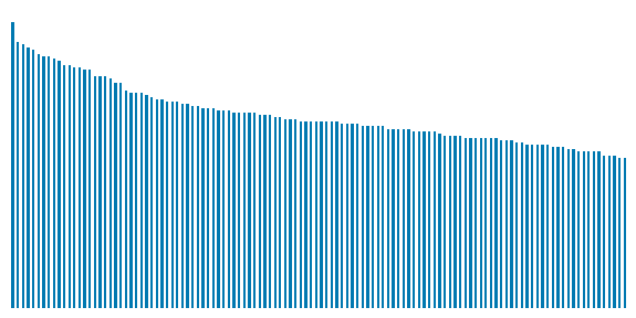
The number of images present in each class

Here we can observe that there is a data imbalance between the classes of different breeds of dogs.

Python3

df['filepath'] = 'train/' + df['id'] + '.jpg'
df.head()

Output:

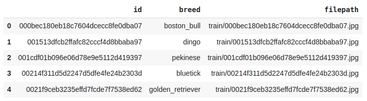
First Five rows of the dataset

Although visualizing one image from each class is not feasible but let’s view some of them.

Python3

plt.subplots(figsize=(10, 10))
for i in range(12):
    plt.subplot(4, 3, i+1)

    # Selecting a random image
    # index from the dataframe.
    k = np.random.randint(0, len(df))
    img = cv2.imread(df.loc[k, 'filepath'])
    plt.imshow(img)
    plt.title(df.loc[k, 'breed'])
    plt.axis('off')
plt.show()

Output:

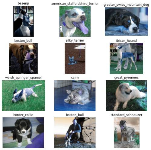
Sample images from the training data

The images are not of the same size which is natural as real-world images tend to be of different sizes and shapes. We will take care of this while loading and processing the images.

Python3

le = LabelEncoder()
df['breed'] = le.fit_transform(df['breed'])
df.head()

Output:

First Five rows of the dataset

Image Input Pipeline

There are times when the dataset is huge and we will be unable to load them into NumPy arrays in one go. Also, we want to apply some custom functions to our images randomly and uniquely such that the images with change do not take up disk space. In such cases image input pipelines build using tf.data.Dataset comes in handy.

Python3

features = df['filepath']
target = df['breed']

X_train, X_val,\
    Y_train, Y_val = train_test_split(features, target,
                                      test_size=0.15,
                                      random_state=10)

X_train.shape, X_val.shape

Output:

((8688,), (1534,))

Below are some of the augmentations which we would like to have in our training data.

Python3

import albumentations as A

transforms_train = A.Compose([
    A.VerticalFlip(p=0.2),
    A.HorizontalFlip(p=0.7),
    A.CoarseDropout(p=0.5),
    A.RandomGamma(p=0.5),
    A.RandomBrightnessContrast(p=1)
])

Let’s view an example of albumentation by applying it to some sample images.

Python3

img = cv2.imread('train/00792e341f3c6eb33663e415d0715370.jpg')
plt.imshow(img)
plt.show()

Output:

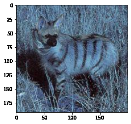
Sample image of a dog

In the above image, we will apply VerticalFlip, HorizontalFlip, CoarseDropout, and CLAHE albumentation technique and check what changes have been done in the image.

Python3

augments = [A.VerticalFlip(p=1), A.HorizontalFlip(p=1),
            A.CoarseDropout(p=1), A.CLAHE(p=1)]

plt.subplots(figsize=(10, 10))
for i, aug in enumerate(augments):
    plt.subplot(2, 2, i+1)
    aug_img = aug(image=img)['image']
    plt.imshow(aug_img)
plt.show()

Output:

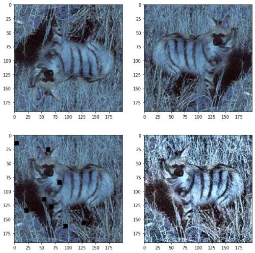
Different data augmentations applied to them

Below we have implemented some utility functions which will be used while building the input pipeline.

• decode_image – This function will read the image from the path and resize them to be of the same size along with it will normalize as well. Finally, we will convert the labels into one_hot vectors as well.
• process_data – This is the function that will be used to introduce image augmentation to the image.

Python3

def aug_fn(img):
    aug_data = transforms_train(image=img)
    aug_img = aug_data['image']

    return aug_img


@tf.function
def process_data(img, label):
    aug_img = tf.numpy_function(aug_fn,
                                [img],
                                Tout=tf.float32)

    return img, label


def decode_image(filepath, label=None):

    img = tf.io.read_file(filepath)
    img = tf.image.decode_jpeg(img)
    img = tf.image.resize(img, [128, 128])
    img = tf.cast(img, tf.float32) / 255.0

    if label == None:
        return img

    return img, tf.one_hot(indices=label,
                           depth=120,
                           dtype=tf.float32)

Now by using the above function we will be implementing our training data input pipeline and the validation data pipeline.

Python3

train_ds = (
    tf.data.Dataset
    .from_tensor_slices((X_train, Y_train))
    .map(decode_image, num_parallel_calls=AUTO)
    .map(partial(process_data), num_parallel_calls=AUTO)
    .batch(32)
    .prefetch(AUTO)
)

val_ds = (
    tf.data.Dataset
    .from_tensor_slices((X_val, Y_val))
    .map(decode_image, num_parallel_calls=AUTO)
    .batch(32)
    .prefetch(AUTO)
)

We must observe here that we do not apply image data augmentation on validation or testing data.

Python3

for img, label in train_ds.take(1):
  print(img.shape, label.shape)

Output:

(32, 128, 128, 3) (32, 120)

From here we can confirm that the images have been converted into (128, 128) shapes and batches of 64 images have been formed.

Model Development

We will use pre-trained weight for an Inception network which is trained on imagenet dataset. This dataset contains millions of images for around 1000 classes of images.

Python3

from tensorflow.keras.applications.inception_v3 import InceptionV3

pre_trained_model = InceptionV3(
    input_shape=(128, 128, 3),
    weights='imagenet',
    include_top=False
)

Output:

87916544/87910968 [==============================] - 1s 0us/step
87924736/87910968 [==============================] - 1s 0us/step

Let’s check how deep or the number of layers are there in this pre-trained model.

Python3

len(pre_trained_model.layers)

Output:

311

This is how deep this model is this also justifies why this model is highly effective in extracting useful features from images which helps us to build classifiers. The parameters of a model we import are already trained on millions of images and for weeks so, we do not need to train them again.

Python3

for layer in pre_trained_model.layers:
  layer.trainable = False

last_layer = pre_trained_model.get_layer('mixed7')
print('last layer output shape: ', last_layer.output_shape)
last_output = last_layer.output

Output:

last layer output shape:  (None, 6, 6, 768)

Model Architecture

We will implement a model using the  Functional API of Keras which will contain the following parts:

• The base model is the Inception model in this case.
• The Flatten layer flattens the output of the base model’s output.
• Then we will have two fully connected layers followed by the output of the flattened layer.
• We have included some BatchNormalization layers to enable stable and fast training and a Dropout layer before the final layer to avoid any possibility of overfitting.
• The final layer is the output layer which outputs soft probabilities for the three classes. 

Python3

# Model Architecture
x = layers.Flatten()(last_output)
x = layers.Dense(256, activation='relu')(x)
x = layers.BatchNormalization()(x)
x = layers.Dense(256, activation='relu')(x)
x = layers.Dropout(0.3)(x)
x = layers.BatchNormalization()(x)
output = layers.Dense(120, activation='softmax')(x)

model = keras.Model(pre_trained_model.input, output)

# Model Compilation
model.compile(
    optimizer='adam',
    loss=keras.losses.CategoricalCrossentropy(from_logits=True),
    metrics=['AUC']
)

Callback

Callbacks are used to check whether the model is improving with each epoch or not. If not then what are the necessary steps to be taken like ReduceLROnPlateau decreasing the learning rate further? Even then if model performance is not improving then training will be stopped by EarlyStopping. We can also define some custom callbacks to stop training in between if the desired results have been obtained early.

Python3

from keras.callbacks import EarlyStopping, ReduceLROnPlateau

class myCallback(tf.keras.callbacks.Callback):
    def on_epoch_end(self, epoch, logs={}):
        if logs.get('val_auc') > 0.99:
            print('\n Validation accuracy has reached upto 90%\
      so, stopping further training.')
            self.model.stop_training = True

es = EarlyStopping(patience=3,
                   monitor='val_auc',
                   restore_best_weights=True)

lr = ReduceLROnPlateau(monitor='val_loss',
                       patience=2,
                       factor=0.5,
                       verbose=1)

Now we will train our model:

Python3

history = model.fit(train_ds,
                    validation_data=val_ds,
                    epochs=50,
                    verbose=1,
                    callbacks=[es, lr, myCallback()])

Output:

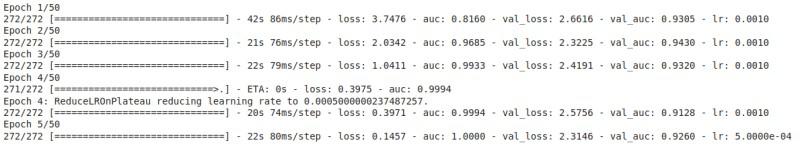
Training and validation loss and AUC score

Let’s visualize the training and validation accuracy with each epoch.

Python3

history_df = pd.DataFrame(history.history)
history_df.loc[:, ['loss', 'val_loss']].plot()
history_df.loc[:, ['auc', 'val_auc']].plot()
plt.show()

Output:

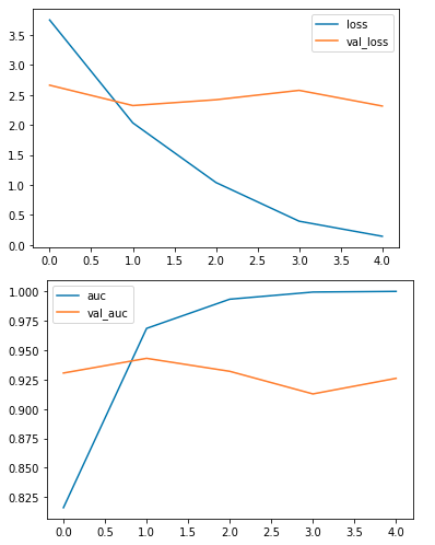
Graph of loss and accuracy epoch by epoch for training and validation data loss

From the above graphs, we can observe that the model has overfitted the training data as the difference between the training and validation AUC score is quite observable.